Alzheimer's Clinical Research Data via R Packages: the Alzverse

Abstract

Sharing clinical research data is essential for advancing research in Alzheimer’s disease (AD) and other therapeutic areas. However, challenges in data accessibility, standardization, documentation, usability, and reproducibility continue to impede this goal. In this article, we highlight the advantages of using R packages to overcome these challenges using two examples. The first example R package, ‘A4LEARN’ includes data from a randomized trial (the Anti-Amyloid Treatment in Asymptomatic Alzheimer’s [A4] study) and its companion observational study of biomarker negative individuals (the Longitudinal Evaluation of Amyloid Risk and Neurodegeneration [LEARN] study). The second example is the ADNIMERGE2 R package, which includes data from the Alzheimer’s Disease Neuroimaging Initiative (ADNI). These packages bundle raw and processed data, documentation, and reproducible analyses into a portable, analysis-ready formats. By promoting collaboration, transparency, and reproducibility, R data packages can play a vital role in accelerating clinical research.

Introduction

Alzheimer’s disease (AD) is one of the leading neurodegenerative diseases worldwide, with growing evidence supporting its multifactorial etiology. The Alzheimer’s Disease Neuroimaging Initiative (ADNI) (Weiner et al. 2025) and similar projects have accumulated vast quantities of clinical, neuroimaging, and biomarker data, creating opportunities for scientific advances in the understanding and treatment of AD. ADNI has provided data for more than 6000 scientific papers publications (Weiner et al. 2025).

Availability of such data is on the rise, due in part to data sharing mandates from funders like the National Institutes of Health. However, it often takes considerable time and effort for researchers to gain sufficient familiarity with the data to produce meaningful analyses. Learning curves can be steep due to inadequate or hard-to-locate documentation and example analysis code.

Open-source software solutions, particularly in the form of R packages (R Core Team 2019; Wickham and Bryan 2023), offer significant potential to address these barriers. The R programming language is widely used in biostatistics, machine learning, and clinical research. R packages are a well-known means for distributing cutting edge statistical software and documentation, and they often include data and analysis vignettes which demonstrate how the methods can be applied to data. But R packages can also be used to share data itself. The authors have maintained the ADNIMERGE R data package since 2017 ((ADNI) 2023). ADNIMERGE has been cited by about 250 articles¹ and has inspired related projects, such as the ANMERGE package of AddNeuroMed Consortium data (Birkenbihl et al. 2021). Vuorre and Crump (2021) demonstrated the utility of R packages for sharing data and analysis code from psychological experiments.

We discuss how R packages can also facilitate easy access, harmonization, and analysis of larger clinical datasets from AD studies. These packages are built with the goal of providing an audit trail of derived data progeny, supporting reproducible research, and leveraging outstanding R tools for unit testing and validation (Wickham 2011), websites (Wickham, Hesselberth, et al. 2024), and regulatory submissions (Knoph and contributors 2023).

In this paper we discuss the advantages of using R packages to share large clinical study datasets, and provide two new examples: the A4LEARN packages which includes data from a randomized trial (the Anti-Amyloid Treatment in Asymptomatic Alzheimer’s [A4] study) (Sperling et al. 2023) and its companion observational study of biomarker negative individuals (the Longitudinal Evaluation of Amyloid Risk and Neurodegeneration [LEARN] study) (Sperling et al. 2024); and the ADNIMERGE2 package, which includes latest data from the Alzheimer’s Disease Neuroimaging Initiative (ADNI) (Weiner et al. 2025).

Advantages of R Data Packages

Reproducibility, Portability and Documentation

The most important advantage of using R data packages for sharing clinical research data, is that it facilitates reproducible research. R is widely available and free to download (R Core Team 2025), commonly used in statistics courses, and has active development communities such as academic statisticians, pharmaceutical statisticians, and commercial enterprises such as Posit’s RStudio Integrated Development Environment (IDE).

All R packages include a manual that details the functions and datasets in a standardized format. This content is linked R object’s name accessible to the R user (e.g. by typing ?t.test, or ?cars) and can be browsed within the IDE. This is a drastic improvement compared to the typical case in which relevant data documentation might be contained in unlinked documents and/or data dictionary spreadsheets. R packages also typically provide analysis “vignettes”, which demonstrate how functions can be applied to available datasets to produce analysis results as tables or figures. These are also linked and can be browsed within the IDE. Our A4LEARN package contains a vignette to exactly reproduce key findings of the published manuscript for the trial (Sperling et al. 2023). This code can be used by outside researchers to jump start their own inquiries, and help ensure the data is being used correctly, efficiently, and consistent with the intentions of the study team.

The R package bundle of data, R functions, documentation and vignettes is made portable as an efficiently compressed file which can be installed on any machine running R. Data files within the package are also efficiently compressed using R’s .RData file format. These .RData files can be read by SPSS, Stata, and SAS [CONFIRM]. Another advantage to .RData compared to tabular text files (e.g. .csv files), is that they can utilize R object classes such as dates and factor variables, eliminating the need to process and annotate data prior to analysis.

The pkgdown R package (Wickham, Hesselberth, et al. 2024) makes it trivial to export documentation and vignettes as a website, and integrates well with code repositories such as GitHub. These pkgdown websites are searchable, and make the documentation and examples available to researchers who do not use R. See atri-biostats.github.io/A4LEARN/ and atri-biostats.github.io/ADNIMERGE2 for examples.

Standardized and Efficient Workflow and Testing

Questions often arise about the original source of data or how derived variables were defined. Therefore, it is crucial to preserve a record of data progeny. The standardize R package structure and build workflow makes it easy to retrace the steps of the package build. R packages also have a standardize framework for testing (Wickham 2011) and tools for “assertive” programming to verify assumptions about the data (Fischetti 2023).

The R package structure and workflow has been well-documented (Wickham and Bryan 2023). We briefly review the structure while highlighting some key aspects in the context of the clinical research data.

data-raw. The data-raw directory is intended to house raw data and code to import and process raw data and store as .Rdata files in the data directory. Raw data can be preserved in the package with minimal manipulation, or it can be processed attaching meta data (variable labels and units), and ensuring factors and dates are stored as the correct object class. Data dictionary spreadsheets can be parsed to provide content for manual pages (Wickham, Danenberg, et al. 2024).

vignettes. The vignettes directory houses the analysis demonstrations, typically as Rmarkdown (.Rmd) files (Allaire et al. 2024). We prefer to create derived datasets and variables as a vignette, as well, so that derivations are easily accessible to researchers within the IDE. These vignettes can include assertive programming to ensure data conforms to expectations (Fischetti 2023). ADNIMERGE2 contains vignettes which use pharmaverse workflows to derive CDISC ADaM datasets.

R. The R directory contains .R files with code defining R functions and manual content (Wickham, Danenberg, et al. 2024). This directory can store scoring functions, which might be necessary to derive scores from item-level data from psychometric assessments, for example.

testthat. The testthat directory includes automated tests that are checked when the package is built. Sensitive and crucial code that requires replication by independent programmers can be tested here, to ensure they produce equivalent results on the actual data and/or test data.

reports. Report code that is not wanted as a vignette can be stored in a separate directory for general reports. Of note, rmarkdown supports “parameterized reports”, which can produce different output depending on the supplied parameter(s). Clinical trials like A4 often include several outcomes collected on the same schedule and analyzed with the same approach. Instead of writing identical code for several outcomes, one generic parameterized rmarkdown file can produce all of these reports. Clinical trial outcomes are often aggregated into one long dataset with a row for each subject, time point, and outcome (see ADQS in the A4LEARN package). The parameterized report can filter this long dataset for the desired outcome and analyze only that outcome. Futhermore, using R parallel programming tools (e.g. Wickham (2023)), these reports can be produced in parallel. In the case of the A4 trial read out, once data from the blinded phase was locked and unblinded it only took about 30 minutes to build the final data package and render all planned analysis reports and summary slide decks.

Example `R` Data Packages

ADNIMERGE2

The ADNIMERGE2 package was built using pharmaverse tools. It can be downloaded from loni.usc.edu. Below are examples of some basic summaries of participant characteristics by phase, or wave, of ADNI can be created using the derived ADSL data table in the package.

tbl_summary(
  data = ADNIMERGE2::ADSL %>%
    filter(ENRLFL %in% "Y"),
  by = ORIGPROT,
  include = c(AGE, SEX, EDUC, RACE, ETHNIC, BMI, DX, APOE, 
    ADASTT13, CDRSB, MMSCORE),
  type = all_continuous() ~ "continuous2",
  statistic = list(
    all_continuous() ~ "{mean} ({sd})",
    all_categorical() ~ "{n} ({p}%)"
  ),
  digits = all_continuous() ~ 1,
  percent = "column",
  missing_text = "(Missing)"
) %>%
  add_overall(last = TRUE) %>%
  add_stat_label(label = all_continuous2() ~ "Mean (SD)") %>%
  modify_footnote_header(
    footnote = "Column-wise percentage; n (%)",
    columns = all_stat_cols(),
    replace = TRUE
  ) %>%
  modify_abbreviation(abbreviation = "ADNI: Alzheimer’s Disease Neuroimaging Initiative; CN: Cognitive Normal; MCI: Mild Cognitive Impairment; DEM: Dementia.") %>%
  modify_caption(
    caption = "Table 1. ADNI - Subject Characteristics by Study Phase"
  ) %>%
  bold_labels()

Table 1. ADNI - Subject Characteristics by Study Phase
Characteristic	ADNI1 N = 819¹	ADNIGO N = 131¹	ADNI2 N = 790¹	ADNI3 N = 696¹	ADNI4 N = 477¹	Overall N = 2,913¹
Age (in Years)
Mean (SD)	75.2 (6.8)	71.6 (7.9)	72.7 (7.2)	70.7 (7.4)	68.7 (7.4)	72.2 (7.6)
Sex, n (%)
Female	342 (42%)	60 (46%)	379 (48%)	381 (55%)	307 (64%)	1,469 (50%)
Male	477 (58%)	71 (54%)	411 (52%)	315 (45%)	170 (36%)	1,444 (50%)
Education
Mean (SD)	15.5 (3.0)	15.8 (2.7)	16.3 (2.6)	16.4 (2.3)	16.0 (2.8)	16.0 (2.7)
(Missing)	1	0	0	0	1	2
Race, n (%)
American Indian or Alaskan Native	1 (0.1%)	1 (0.8%)	1 (0.1%)	2 (0.3%)	3 (0.6%)	8 (0.3%)
Asian	14 (1.7%)	1 (0.8%)	14 (1.8%)	29 (4.2%)	45 (9.4%)	103 (3.5%)
Black or African American	39 (4.8%)	4 (3.1%)	34 (4.3%)	105 (15%)	158 (33%)	340 (12%)
Native Hawaiian or Other Pacific Islander	0 (0%)	0 (0%)	2 (0.3%)	1 (0.1%)	0 (0%)	3 (0.1%)
Other Pacific Islander	0 (0%)	0 (0%)	0 (0%)	0 (0%)	2 (0.4%)	2 (<0.1%)
White	762 (93%)	118 (90%)	728 (92%)	537 (77%)	237 (50%)	2,382 (82%)
More than one race	3 (0.4%)	5 (3.8%)	10 (1.3%)	13 (1.9%)	22 (4.6%)	53 (1.8%)
Unknown	0 (0%)	2 (1.5%)	1 (0.1%)	9 (1.3%)	10 (2.1%)	22 (0.8%)
Ethnicity, n (%)
Hispanic or Latino	19 (2.3%)	8 (6.1%)	31 (3.9%)	58 (8.3%)	66 (14%)	182 (6.2%)
Not Hispanic or Latino	794 (97%)	122 (93%)	755 (96%)	637 (92%)	409 (86%)	2,717 (93%)
Unknown	6 (0.7%)	1 (0.8%)	4 (0.5%)	1 (0.1%)	2 (0.4%)	14 (0.5%)
Body Mass Index
Mean (SD)	27.6 (4.1)	24.0 (NA)	30.8 (7.2)	30.0 (NA)	29.3 (6.5)	29.2 (6.2)
(Missing)	815	130	784	695	450	2,874
Baseline Diagnostics Status, n (%)
CN	225 (29%)	1 (1.0%)	295 (37%)	380 (55%)	292 (61%)	1,193 (42%)
MCI	373 (48%)	99 (99%)	344 (44%)	243 (35%)	148 (31%)	1,207 (42%)
DEM	182 (23%)	0 (0%)	151 (19%)	73 (10%)	37 (7.8%)	443 (16%)
(Missing)	39	31	0	0	0	70
APOE Genotype, n (%)
ε2/ε2	2 (0.2%)	0 (0%)	3 (0.4%)	1 (0.1%)	2 (1.7%)	8 (0.3%)
ε2/ε3	53 (6.5%)	9 (7.0%)	66 (8.5%)	52 (7.7%)	6 (5.1%)	186 (7.4%)
ε2/ε4	18 (2.2%)	2 (1.6%)	14 (1.8%)	17 (2.5%)	4 (3.4%)	55 (2.2%)
ε3/ε3	363 (44%)	67 (52%)	352 (45%)	347 (52%)	53 (45%)	1,182 (47%)
ε3/ε4	295 (36%)	42 (33%)	269 (35%)	204 (30%)	46 (39%)	856 (34%)
ε4/ε4	88 (11%)	8 (6.3%)	75 (9.6%)	52 (7.7%)	7 (5.9%)	230 (9.1%)
(Missing)	0	3	11	23	359	396
Baseline ADAS-Cog Item 13 Total Score
Mean (SD)	18.4 (9.2)	12.4 (5.4)	16.1 (10.1)	13.1 (8.9)	13.0 (8.1)	15.4 (9.4)
(Missing)	8	1	7	11	39	66
Baseline CDR Sum of Boxes Score
Mean (SD)	1.8 (1.8)	1.2 (0.7)	1.5 (1.9)	1.0 (1.6)	0.9 (1.5)	1.4 (1.7)
(Missing)	2	0	0	0	0	2
Baseline MMSE Score
Mean (SD)	26.7 (2.7)	28.3 (1.5)	27.4 (2.7)	28.0 (2.5)	27.9 (2.4)	27.5 (2.6)
(Missing)	2	0	0	0	3	5
Abbreviation: ADNI: Alzheimer’s Disease Neuroimaging Initiative; CN: Cognitive Normal; MCI: Mild Cognitive Impairment; DEM: Dementia.
¹ Column-wise percentage; n (%)

# Prepare analysis dataset of ADAS-cog item-13 score
ADADAS <- ADNIMERGE2::ADQS %>%
  # Enrolled participant
  filter(ENRLFL %in% "Y") %>%
  # ADAS-cog item-13 total score
  filter(PARAMCD %in% "ADASTT13") %>%
  mutate(TIME = convert_number_days(ADY, unit = 'year')) %>%
  filter(!if_any(all_of(c("TIME", "DX", "AVAL")), ~ is.na(.x)))

# Individual profile (spaghetti) plot
ggplot(ADADAS, aes(x = TIME, y = AVAL, group = USUBJID, color = DX)) +
  geom_line(alpha = 0.5) +
  scale_color_manual(values = c("#73C186", "#F2B974", "#DF957C", "#999999")) +
  labs(
    y = "ADAS-cog13 Total Score",
    x = "Years since baseline visit",
    color = "Baseline Diagnostics Status") +
  theme(legend.position = "bottom") +
  guides(colour = guide_legend(override.aes = list(alpha = 1)))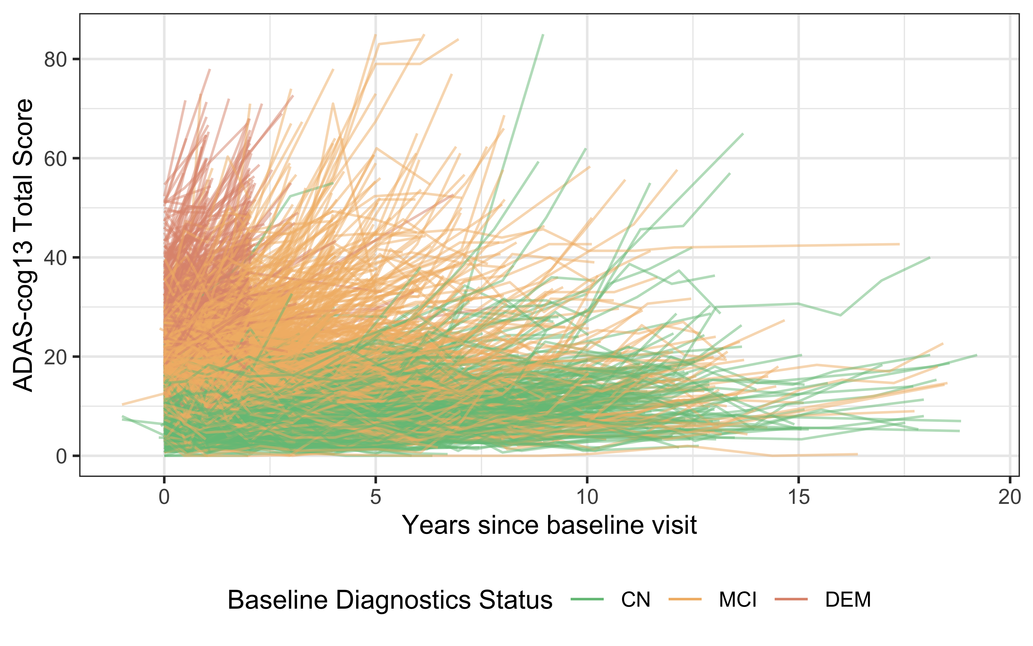

Figure 1. Spahetti plot of ADAS-cog13 scores in ADNI by baseline clinical diagnosis.

A4LEARN

Similarly, A4LEARN data can be easily summarized

tbl_summary(
  data = A4LEARN::SUBJINFO %>% filter(SUBSTUDY != 'SF'),
  by = SUBSTUDY,
  label = SUBJINFO_labels,
  include = c(AGEYR, SEX, EDCCNTU, RACE, ETHNIC, BMIBL, SUBSTUDY, APOEGN, 
    PACCV6, MMSETSV6, AMYLCENT),
  type = all_continuous() ~ "continuous2",
  statistic = list(
    all_continuous() ~ "{mean} ({sd})",
    all_categorical() ~ "{n} ({p}%)"
  ),
  digits = all_continuous() ~ 1,
  percent = "column",
  missing_text = "(Missing)"
) %>%
  add_overall(last = TRUE) %>%
  add_stat_label(label = all_continuous2() ~ "Mean (SD)") %>%
  modify_footnote_header(
    footnote = "Column-wise percentage; n (%)",
    columns = all_stat_cols(),
    replace = TRUE
  ) %>%
  modify_abbreviation(abbreviation = "A4: Anti-Amyloid Treatment in Asymptomatic Alzheimer’s study; LEARN: Longitudinal Evaluation of Amyloid Risk and Neurodegeneration.") %>%
  modify_caption(
    caption = "Table 2. A4 and LEARN - Subject Characteristics by substudy."
  ) %>%
  bold_labels()

Table 2. A4 and LEARN - Subject Characteristics by substudy.
Characteristic	A4 N = 1,169¹	LEARN N = 538¹	Overall N = 1,707¹
Age in years at Consent
Mean (SD)	71.9 (4.8)	70.5 (4.3)	71.5 (4.7)
Sex, n (%)
Male	475 (41%)	208 (39%)	683 (40%)
Female	694 (59%)	330 (61%)	1,024 (60%)
Years of education
Mean (SD)	16.6 (2.8)	16.8 (2.6)	16.6 (2.8)
Race, n (%)
American Indian or Alaskan Native	2 (0.2%)	5 (0.9%)	7 (0.4%)
Asian	24 (2.1%)	12 (2.2%)	36 (2.1%)
Black or African American	28 (2.4%)	14 (2.6%)	42 (2.5%)
More than one race	8 (0.7%)	5 (0.9%)	13 (0.8%)
Unknown or Not Reported	7 (0.6%)	1 (0.2%)	8 (0.5%)
White	1,100 (94%)	501 (93%)	1,601 (94%)
Ethnicity, n (%)
Hispanic or Latino	34 (2.9%)	18 (3.3%)	52 (3.0%)
Not Hispanic or Latino	1,124 (96%)	516 (96%)	1,640 (96%)
Unknown or Not reported	11 (0.9%)	4 (0.7%)	15 (0.9%)
body mass index (weight (kg) / [height (m)]^2)
Mean (SD)	27.4 (5.1)	27.6 (4.9)	27.4 (5.0)
(Missing)	2	1	3
APOE4 genotype (ε2/ε4, ε3/ε4, ε4/ε4, no ε4), n (%)
E2/E2	2 (0.2%)	5 (0.9%)	7 (0.4%)
E2/E3	61 (5.2%)	66 (12%)	127 (7.4%)
E2/E4	35 (3.0%)	10 (1.9%)	45 (2.6%)
E3/E3	417 (36%)	342 (64%)	759 (45%)
E3/E4	560 (48%)	111 (21%)	671 (39%)
E4/E4	94 (8.0%)	2 (0.4%)	96 (5.6%)
(Missing)	0	2	2
PACC Total Score at Visit 6
Mean (SD)	0.0 (2.7)	NA (NA)	0.0 (2.7)
(Missing)	0	538	538
MMSE Total Score at Visit 6, n (%)
22	1 (<0.1%)	0 (NA%)	1 (<0.1%)
24	5 (0.4%)	0 (NA%)	5 (0.4%)
25	25 (2.1%)	0 (NA%)	25 (2.1%)
26	36 (3.1%)	0 (NA%)	36 (3.1%)
27	103 (8.8%)	0 (NA%)	103 (8.8%)
28	229 (20%)	0 (NA%)	229 (20%)
29	347 (30%)	0 (NA%)	347 (30%)
30	419 (36%)	0 (NA%)	419 (36%)
(Missing)	4	538	542
Amyloid PET centiloids. AMYLCENT = 183.07 x SUVRCER – 177.26.
Mean (SD)	66.1 (32.8)	4.2 (12.6)	46.6 (40.2)
Abbreviation: A4: Anti-Amyloid Treatment in Asymptomatic Alzheimer’s study; LEARN: Longitudinal Evaluation of Amyloid Risk and Neurodegeneration.
¹ Column-wise percentage; n (%)

Merging A4, LEARN, and ADNI

ADQS_meta <- ADNIMERGE2::ADQS %>%
  filter(ENRLFL %in% "Y") %>%
  bind_rows(A4LEARN::ADQS %>%
    select(STUDYID = SUBSTUDY, USUBJID = BID, PARAMCD = QSTESTCD, 
      AVAL = QSSTRESN, ADY = QSDTC_DAYS_T0)) %>%
  mutate(TIME = convert_number_days(ADY, unit = 'year'))

ADQS_meta %>%
  filter(DX == 'CN' | STUDYID %in% c('A4', 'LEARN'), 
    PARAMCD %in% c('MMSCORE', 'MMSE')) %>%
ggplot(aes(x = TIME, y = AVAL, color = STUDYID)) +
  geom_line(aes(group = USUBJID), alpha = 0.25) +
  labs(
    y = "MMSE Total Score",
    x = "Years since baseline visit",
    color = "Study") +
  theme(legend.position = "bottom") +
  guides(colour = guide_legend(override.aes = list(alpha = 1)))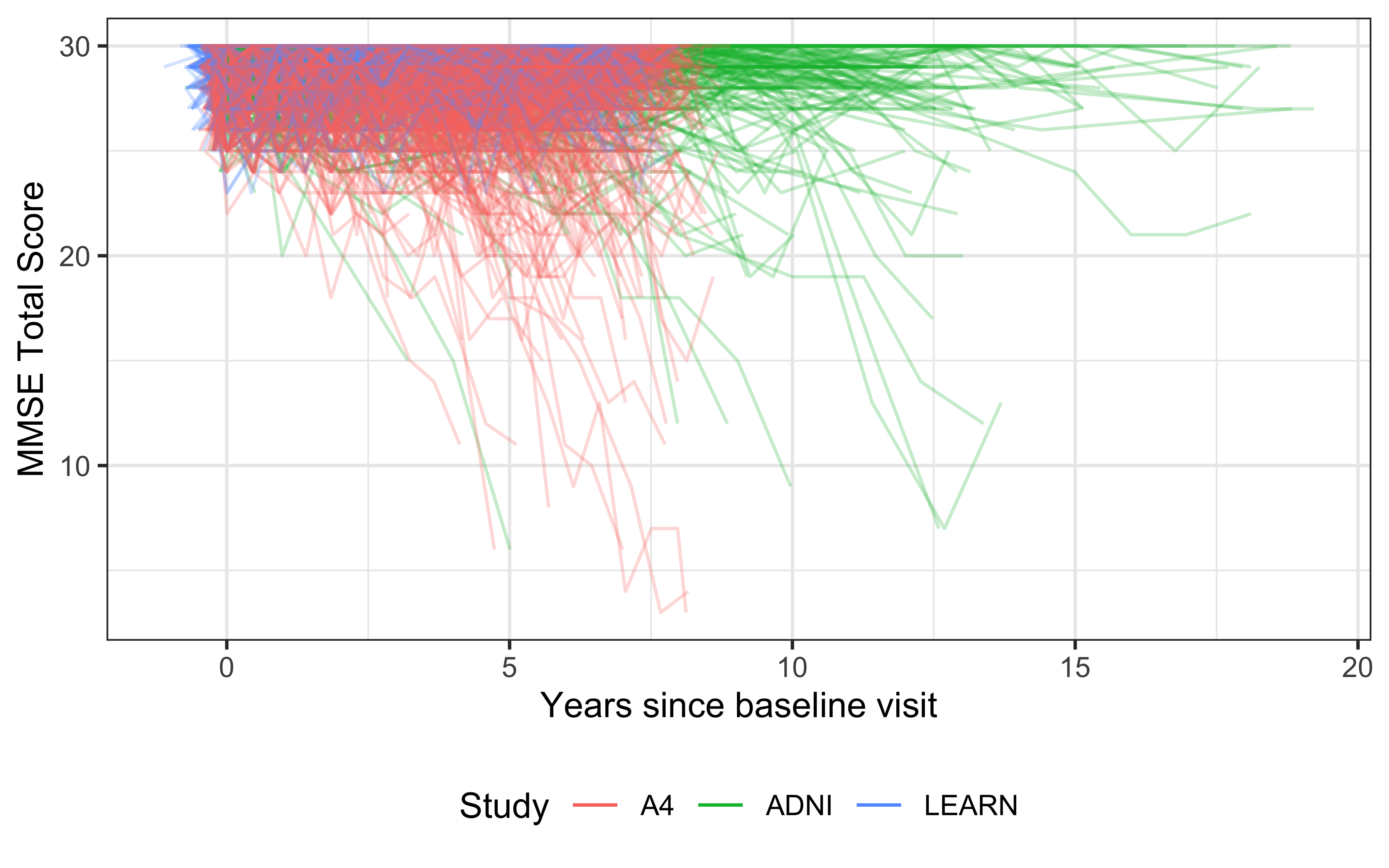

Figure 2. Spahetti plot of MMSE scores in ADNI CN, A4, and LEARN.

Discussion

The development of A4LEARN and ADNIMERGE2 represents a step forward in enabling the Alzheimer’s disease research community to share and analyze data more effectively, and serve as a template for additional future study packages. These packages facilitate the transition from proprietary software like SAS to open-source tools, allowing greater flexibility and transparency in the research process. The shift from SAS to R represents a broader trend in the clinical research community toward open-source and reproducible research practices.

Challenges remain, particularly in the area of data access. In our examples data packages can be sourced using the existing data access models. This puts the onus on data users to go to different sites to obtain data. Once retrieved, The use of locally installed packages poses potential risks, which can be mitigated by using containerization and package management tools like Docker and renv for version control.

Methods

The primary data sources for the packages are derived from the Alzheimer’s Disease Neuroimaging Initiative (ADNI) the A4 and LEARN companions studies. These datasets include longitudinal clinical and neuroimaging data, cognitive test scores, genetic and biomarker data, and other modalities that have been harmonized to facilitate cross-study comparisons.

To ensure usability and consistency, we curated the datasets by mapping variables to standardized terminologies (e.g., CDISC ADaM, SDTM), handling missing data through imputation techniques, and deriving key analysis variables.

A4LEARN and ADNIMERGE2 were developed using best practices in R package development, including:

R Package Architecture: Each package is modular, supporting various stages of data analysis, from raw data processing to the generation of regulatory-compliant datasets.
Data Standardization: The packages support standardization of clinical data, with built-in functions to harmonize variable formats, handle missing values, and generate standardized metadata.
Reproducibility: Built-in vignettes and examples guide users through the installation, data loading, and analysis processes. The packages integrate with tools like renv and Docker to facilitate reproducibility in different computing environments.

The R package framework facilitates the creation of Analysis Data Model (ADaM) datasets, which are the gold standard for statistical analysis in clinical trials. The admiral package is used to generate ADaM datasets for ADNIMERGE2. Other pharmaverse tools can be used to create regulatory-compliant tables, listings, and figures.

Data Availability

Data is available from:

A4LEARN: A4StudyData.org
ADNIMERGE2: loni.usc.edu

Data documentation is available from

A4LEARN: atri-biostats.github.io/A4LEARN/
ADNIMERGE2: atri-biostats.github.io/ADNIMERGE2

Code Availability

R code is available for download from the following repositories:

alzverse: github.com/atri-biostats/alzverse
A4LEARN: github.com/atri-biostats/A4LEARN
ADNIMERGE2: github.com/atri-biostats/ADNIMERGE2

Author Contributions

Competing Interests

Acknowledgements

References

(ADNI), Alzheimer’s Disease Neuroimaging Initiative. 2023. “ADNI Data Archive.” https://adni.loni.usc.edu/support/.

Allaire, JJ, Yihui Xie, Christophe Dervieux, Jonathan McPherson, Javier Luraschi, Kevin Ushey, Aron Atkins, et al. 2024. Rmarkdown: Dynamic Documents for r. https://github.com/rstudio/rmarkdown.

Birkenbihl, Colin, Sarah Westwood, Liu Shi, Alejo Nevado-Holgado, Eric Westman, Simon Lovestone, AddNeuroMed Consortium, and Martin Hofmann-Apitius. 2021. “ANMerge: A Comprehensive and Accessible Alzheimer’s Disease Patient-Level Dataset.” Journal of Alzheimer’s Disease 79 (1): 423–31.

Fischetti, Tony. 2023. Assertr: Assertive Programming for r Analysis Pipelines. https://doi.org/10.32614/CRAN.package.assertr.

Knoph, Ari Siggaard, and pharmaverse contributors. 2023. Pharmaverse: Navigate ’Pharmaverse’. https://doi.org/10.32614/CRAN.package.pharmaverse.

R Core Team. 2019. R: A Language and Environment for Statistical Computing. Vienna, Austria: R Foundation for Statistical Computing. https://www.R-project.org.

———. 2025. R: A Language and Environment for Statistical Computing. Vienna, Austria: R Foundation for Statistical Computing. https://www.R-project.org/.

Sperling, Reisa A, MC Donohue, RA Rissman, KA Johnson, DM Rentz, JD Grill, JL Heidebrink, et al. 2024. “Amyloid and Tau Prediction of Cognitive and Functional Decline in Unimpaired Older Individuals: Longitudinal Data from the A4 and LEARN Studies.” The Journal of Prevention of Alzheimer’s Disease 11 (4): 802–13.

Sperling, Reisa A, Michael C Donohue, Rema Raman, Michael S Rafii, Keith Johnson, Colin L Masters, Christopher H van Dyck, et al. 2023. “Trial of Solanezumab in Preclinical Alzheimer’s Disease.” New England Journal of Medicine 389 (12): 1096–1107.

Vuorre, Matti, and Matthew JC Crump. 2021. “Sharing and Organizing Research Products as r Packages.” Behavior Research Methods 53: 792–802.

Weiner, Michael W, Shaveta Kanoria, Melanie J Miller, Paul S Aisen, Laurel A Beckett, Catherine Conti, Adam Diaz, et al. 2025. “Overview of Alzheimer’s Disease Neuroimaging Initiative and Future Clinical Trials.” Alzheimer’s & Dementia 21 (1): e14321.

Wickham, Hadley. 2011. “Testthat: Get Started with Testing.” The R Journal 3: 5–10. https://journal.r-project.org/archive/2011-1/RJournal_2011-1_Wickham.pdf.

———. 2023. Multidplyr: A Multi-Process ’Dplyr’ Backend. https://doi.org/10.32614/CRAN.package.multidplyr.

Wickham, Hadley, and Jennifer Bryan. 2023. R Packages. " O’Reilly Media, Inc.".

Wickham, Hadley, Peter Danenberg, Gábor Csárdi, and Manuel Eugster. 2024. Roxygen2: In-Line Documentation for r. https://doi.org/10.32614/CRAN.package.roxygen2.

Wickham, Hadley, Jay Hesselberth, Maëlle Salmon, Olivier Roy, and Salim Brüggemann. 2024. Pkgdown: Make Static HTML Documentation for a Package. https://doi.org/10.32614/CRAN.package.pkgdown.

Michael C. Donohue, Kedir Hussen, Oliver Langford, Richard Armenta, Gustavo Jimenez-Maggiora

7 August 2025

Abstract

Introduction

Advantages of R Data Packages

Reproducibility, Portability and Documentation

Standardized and Efficient Workflow and Testing

Example `R` Data Packages

ADNIMERGE2

A4LEARN

Merging A4, LEARN, and ADNI

Discussion

Methods

Data Availability

Code Availability

Author Contributions

Competing Interests

Acknowledgements

References

Alzheimer's Clinical Research Data via R Packages: the Alzverse

Michael C. Donohue, Kedir Hussen, Oliver Langford, Richard Armenta, Gustavo Jimenez-Maggiora

7 August 2025

Abstract

Introduction

Advantages of R Data Packages

Reproducibility, Portability and Documentation

Standardized and Efficient Workflow and Testing

Example R Data Packages

ADNIMERGE2

A4LEARN

Merging A4, LEARN, and ADNI

Discussion

Methods

Data Availability

Code Availability

Author Contributions

Competing Interests

Acknowledgements

References

Example `R` Data Packages