A4 Primary Results
ATRI Biostatistics
Source:vignettes/A4-Primary-Results.Rmd
A4-Primary-Results.RmdThe Anti-Amyloid Treatment in Asymptomatic Alzheimer’s Disease (A4) study was a Phase 3, double-blind, placebo-controlled study of solanezumab in subjects with preclinical Alzheimer’s Disease (Sperling et al. 2023). The code below demonstrates how to reproduce some primary findings of the A4 trial (Sperling et al. 2023) using R Core Team (2024). Data were downloaded from https://www.a4studydata.org/ on 2025-08-08.
Load required R packages
library(tidyverse)
library(arsenal)
library(kableExtra)
library(nlme)
library(emmeans)
library(splines)
library(clubSandwich)
library(A4LEARN)

formatp <- function(x) case_when(
  x < 0.001 ~ "p<0.001",
  x > 0.01 ~ Hmisc::format.pval(x, digits=2, eps=0.01, nsmall=2),
  TRUE ~ Hmisc::format.pval(x, digits=3, eps=0.001, nsmall=3))
Organize data
# Outcomes collected at Visit 1
V1OUTCOME <- A4LEARN::ADQS %>%
  dplyr::filter(VISITCD == "001") %>%
  select(BID, QSTESTCD, QSSTRESN) %>%
  pivot_wider(values_from = QSSTRESN, names_from = QSTESTCD)

# Outcomes collected at Visit 6
V6OUTCOME <- A4LEARN::ADQS %>%
  dplyr::filter(VISITCD == "006") %>%
  select(BID, QSTESTCD, QSSTRESN) %>%
  pivot_wider(values_from = QSSTRESN, names_from = QSTESTCD)

SUBJINFO <- A4LEARN::SUBJINFO %>%
  left_join(V6OUTCOME, by = "BID") %>%
  left_join(V1OUTCOME %>%
      select(BID, CDRSB, CFITOTAL, CFISP, CFIPT, ADLPQPT, ADLPQSP),
    by = "BID")

# Filter A4LEARN::ADQS for PACC collected in the blinded phases among mITT population
ADQS_PACC <- A4LEARN::ADQS %>%
  dplyr::filter(MITTFL== 1) %>%
  dplyr::filter(EPOCH == "BLINDED TREATMENT" | AVISIT == "006") %>%
  dplyr::filter(QSTESTCD == "PACC") %>%
  rename(PACC = QSSTRESN) %>%
  select(BID, ASEQNCS, TX, ADURW, TX, AGEYR,
    AAPOEGNPRSNFLG, EDCCNTU, SUVRCER, QSVERSION, PACC) %>%
  mutate(TX = factor(TX, levels = c("Placebo", "Solanezumab"))) %>%
  arrange(BID, ADURW) %>%
  na.omit()
Baseline characteristics of the A4 trial
A4labels <- list(TX = "Treatment group", AGEYR = "Age (y)",
  EDCCNTU = "Education (y)", SUVRCER = "FBP SUVr", AMYLCENT = "FBP Centiloid",
  LMIIa = "LM Delayed Recall",  MMSE = "MMSE",
  CFITOTAL = "CFI Combined", ADLPQSP = "ADL Partner", CDRSB = "CDR-SB",
  SEX = "Sex", RACE = "Racial categories", ETHNIC = "Ethnicity",
  MARITAL = "Marital Status",  WRKRET = "Retirement Status",
  APOEGNPRSNFLG = "APOE e4", APOEGN = "APOE Genotype")

table1 <- tableby(TX ~ AGEYR + EDCCNTU + SEX + RACE + ETHNIC + MARITAL + WRKRET +
    SUVRCER + AMYLCENT + chisq(APOEGN) + chisq(APOEGNPRSNFLG) +
    PACC + LMIIa + MMSE + CFITOTAL + ADLPQSP + CDRSB,
  data = SUBJINFO %>% dplyr::filter(MITTFL== 1),
  control = tableby.control(test=TRUE,
    stats.labels = list(Nmiss = "Missing")))

summary(table1, labelTranslations = A4labels, digits = 1,
title = "Characteristics of the A4 participants by randomized treatment group (Modified Intention-to-Treat Population of those who received at least one dose of solanezumab or placebo and underwent assessment for the primary end point).")| Placebo (N=583) | Solanezumab (N=564) | Total (N=1147) | p value | |
|---|---|---|---|---|
| Age (y) | 0.923 | |||
| Mean (SD) | 71.9 (5.0) | 72.0 (4.7) | 72.0 (4.8) | |
| Range | 65.0 - 85.7 | 65.0 - 85.5 | 65.0 - 85.7 | |
| Education (y) | 0.785 | |||
| Mean (SD) | 16.6 (2.9) | 16.6 (2.7) | 16.6 (2.8) | |
| Range | 8.0 - 30.0 | 7.0 - 30.0 | 7.0 - 30.0 | |
| Sex | 0.481 | |||
| Male | 231 (39.6%) | 235 (41.7%) | 466 (40.6%) | |
| Female | 352 (60.4%) | 329 (58.3%) | 681 (59.4%) | |
| Racial categories | 0.831 | |||
| American Indian or Alaskan Native | 0 (0.0%) | 1 (0.2%) | 1 (0.1%) | |
| Asian | 13 (2.2%) | 11 (2.0%) | 24 (2.1%) | |
| Black or African American | 15 (2.6%) | 12 (2.1%) | 27 (2.4%) | |
| More than one race | 3 (0.5%) | 5 (0.9%) | 8 (0.7%) | |
| Unknown or Not Reported | 3 (0.5%) | 4 (0.7%) | 7 (0.6%) | |
| White | 549 (94.2%) | 531 (94.1%) | 1080 (94.2%) | |
| Ethnicity | 0.910 | |||
| Hispanic or Latino | 18 (3.1%) | 16 (2.8%) | 34 (3.0%) | |
| Not Hispanic or Latino | 560 (96.1%) | 542 (96.1%) | 1102 (96.1%) | |
| Unknown or Not reported | 5 (0.9%) | 6 (1.1%) | 11 (1.0%) | |
| Marital Status | 0.208 | |||
| Divorced | 80 (13.7%) | 89 (15.8%) | 169 (14.7%) | |
| Married | 415 (71.2%) | 405 (71.8%) | 820 (71.5%) | |
| Never married | 26 (4.5%) | 14 (2.5%) | 40 (3.5%) | |
| Unknown or Not Reported | 12 (2.1%) | 6 (1.1%) | 18 (1.6%) | |
| Widowed | 50 (8.6%) | 50 (8.9%) | 100 (8.7%) | |
| Retirement Status | 0.722 | |||
| No | 142 (24.4%) | 126 (22.3%) | 268 (23.4%) | |
| Not Applicable | 9 (1.5%) | 9 (1.6%) | 18 (1.6%) | |
| Yes | 432 (74.1%) | 429 (76.1%) | 861 (75.1%) | |
| FBP SUVr | 0.903 | |||
| Mean (SD) | 1.3 (0.2) | 1.3 (0.2) | 1.3 (0.2) | |
| Range | 1.0 - 2.1 | 1.0 - 2.1 | 1.0 - 2.1 | |
| FBP Centiloid | 0.903 | |||
| Mean (SD) | 65.9 (32.1) | 66.2 (33.5) | 66.0 (32.8) | |
| Range | 0.3 - 205.4 | 0.3 - 201.7 | 0.3 - 205.4 | |
| APOE Genotype | 0.624 | |||
| E2/E2 | 0 (0.0%) | 1 (0.2%) | 1 (0.1%) | |
| E2/E3 | 33 (5.7%) | 28 (5.0%) | 61 (5.3%) | |
| E2/E4 | 22 (3.8%) | 13 (2.3%) | 35 (3.1%) | |
| E3/E3 | 208 (35.7%) | 202 (35.8%) | 410 (35.7%) | |
| E3/E4 | 273 (46.8%) | 273 (48.4%) | 546 (47.6%) | |
| E4/E4 | 47 (8.1%) | 47 (8.3%) | 94 (8.2%) | |
| APOE e4 | 0.896 | |||
| No | 241 (41.3%) | 231 (41.0%) | 472 (41.2%) | |
| Yes | 342 (58.7%) | 333 (59.0%) | 675 (58.8%) | |
| PACC | 0.831 | |||
| Mean (SD) | -0.0 (2.6) | 0.0 (2.7) | 0.0 (2.7) | |
| Range | -12.5 - 7.8 | -10.3 - 6.4 | -12.5 - 7.8 | |
| LM Delayed Recall | 0.757 | |||
| Missing | 1 | 0 | 1 | |
| Mean (SD) | 12.7 (3.5) | 12.6 (3.8) | 12.6 (3.7) | |
| Range | 2.0 - 22.0 | 0.0 - 23.0 | 0.0 - 23.0 | |
| MMSE | 0.763 | |||
| Mean (SD) | 28.8 (1.2) | 28.8 (1.3) | 28.8 (1.3) | |
| Range | 24.0 - 30.0 | 22.0 - 30.0 | 22.0 - 30.0 | |
| CFI Combined | 0.045 | |||
| Missing | 2 | 0 | 2 | |
| Mean (SD) | 3.6 (3.3) | 4.0 (3.6) | 3.8 (3.5) | |
| Range | 0.0 - 20.0 | 0.0 - 22.0 | 0.0 - 22.0 | |
| ADL Partner | 0.266 | |||
| Mean (SD) | 43.5 (2.6) | 43.4 (2.7) | 43.4 (2.6) | |
| Range | 26.8 - 45.0 | 25.0 - 45.0 | 25.0 - 45.0 | |
| CDR-SB | 0.154 | |||
| Mean (SD) | 0.0 (0.2) | 0.1 (0.2) | 0.1 (0.2) | |
| Range | 0.0 - 2.0 | 0.0 - 1.0 | 0.0 - 2.0 |
Primary analyis of the PACC
Preclinical Alzheimer Cognitive Composite (PACC, Donohue et al. (2014)) data was modeled using natural cubic splines as described in Donohue et al. (2023). The fixed effects included the following terms: (i) spline basis expansion terms (two terms), (ii) spline basis expansion terms-by-treatment interaction (two terms), (iii) PACC test version administered, (iv) baseline age, (v) education, (vi) APOE4 Carrier Status (yes/no), and (vii) baseline florbetapir cortical SUVr. The model is constrained to not allow a difference between treatment group means at baseline. The following variance-covariance structures were assumed in sequence until a model converged: (i) heterogeneous unstructured, (ii) heterogeneous Toeplitz, (iii) heterogeneous autoregressive order 1, (iv) heterogeneous compound symmetry, and (v) compound symmetry. The first structure, heterogeneous unstructured, did not converge. Here we fit the second, heterogeneous Toeplitz, which did converge.
ggplot(ADQS_PACC, aes(x=ADURW, y=PACC, color=TX)) +
  geom_line(aes(group = BID), alpha=0.2) +
  theme(legend.position = "inside", legend.position.inside = c(0.2, 0.2)) +
  xlab("Weeks since Randomization") +
  scale_x_continuous(breaks = seq(0, max(ADQS_PACC$ADURW), by = 24))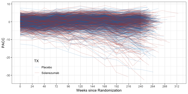
Spaghetti plot of PACC data over time by treatment group.
# Spline basis expansion functions
# CAUTION: these function depend on the ADQS_PACC data frame object in the
# global environment. If ADQS_PACC changes, so do these funtions
ns21 <- function(t){
  as.numeric(predict(splines::ns(ADQS_PACC$ADURW, df=2,
    Boundary.knots = c(0, max(ADQS_PACC$ADURW))), t)[,1])
}
ns22 <- function(t){
  as.numeric(predict(splines::ns(ADQS_PACC$ADURW, df=2,
    Boundary.knots = c(0, max(ADQS_PACC$ADURW))), t)[,2])
}

assign("ns21", ns21, envir = .GlobalEnv)
assign("ns22", ns22, envir = .GlobalEnv)

# GLS model fit:
pacc_fit <- gls(PACC ~
    I(ns21(ADURW)) + I(ns22(ADURW)) +
    (I(ns21(ADURW)) + I(ns22(ADURW))):TX +
    AGEYR + AAPOEGNPRSNFLG + EDCCNTU + SUVRCER + QSVERSION,
  data = ADQS_PACC,
  weights = varIdent(form = ~ 1 | ASEQNCS),
  correlation = corARMA(form = ~ ASEQNCS | BID, p = 10))
ref_grid(pacc_fit,
  at = list(ADURW = c(0,240), TX = levels(ADQS_PACC$TX)),
  vcov. = clubSandwich::vcovCR(pacc_fit, type = "CR2") %>% as.matrix(),
  data = ADQS_PACC,
  mode = "satterthwaite") %>%
  emmeans(~ ADURW | TX) %>%
  pairs(reverse = TRUE) %>%
  as_tibble() %>%
  mutate(p.value = formatp(p.value)) %>%
  kable(caption = "Mean PACC change from baseline at week 240 by treatment
    group estimated from spline model.", digits = 2, booktabs = TRUE) %>%
kableExtra::kable_styling(latex_options = "HOLD_position")| contrast | TX | estimate | SE | df | t.ratio | p.value |
|---|---|---|---|---|---|---|
| ADURW240 - ADURW0 | Placebo | -1.13 | 0.16 | 10791 | -6.88 | p<0.001 |
| ADURW240 - ADURW0 | Solanezumab | -1.43 | 0.21 | 10791 | -6.95 | p<0.001 |
contrast240 <- ref_grid(pacc_fit,
  at = list(ADURW = 240, TX = levels(ADQS_PACC$TX)),
  vcov. = clubSandwich::vcovCR(pacc_fit, type = "CR2") %>% as.matrix(),
  data = ADQS_PACC,
  mode = "satterthwaite") %>%
  emmeans(specs = "TX", by = "ADURW") %>%
  pairs(reverse = TRUE, adjust = "none")

contrast240 %>%
  as_tibble() %>%
  left_join(contrast240 %>%
      confint() %>%
      as_tibble() %>%
      select(contrast, lower.CL, upper.CL), by="contrast") %>%
  relocate(p.value, .after = last_col()) %>%
  mutate(p.value = formatp(p.value)) %>%
  kable(caption = "Mean PACC group change from baseline at week 240 by treatment
    group estimated from spline model.", digits = 2, booktabs = TRUE) %>%
kableExtra::kable_styling(latex_options = "HOLD_position")| contrast | ADURW | estimate | SE | df | t.ratio | lower.CL | upper.CL | p.value |
|---|---|---|---|---|---|---|---|---|
| Solanezumab - Placebo | 240 | -0.3 | 0.26 | 10791 | -1.13 | -0.82 | 0.22 | 0.26 |
ref_grid(pacc_fit,
  at = list(ADURW = seq(0, 312, by=12), TX = levels(ADQS_PACC$TX)),
  vcov. = clubSandwich::vcovCR(pacc_fit, type = "CR2") %>% as.matrix(),
  data = ADQS_PACC,
  mode = "satterthwaite") %>%
  emmeans(specs = "TX", by = "ADURW") %>%
  as_tibble() %>%
  ggplot(aes(x=ADURW, y=emmean)) +
  geom_line(aes(color=TX)) +
  geom_ribbon(aes(ymin = lower.CL, ymax = upper.CL, fill = TX), alpha = 0.2) +
  scale_x_continuous(breaks = seq(0, 312, by=24)) +
  ylab("Mean PACC with 95% confidence intervals") +
  xlab("Weeks since Randomization") +
  theme(legend.position = 'inside', legend.position.inside = c(0.2, 0.2))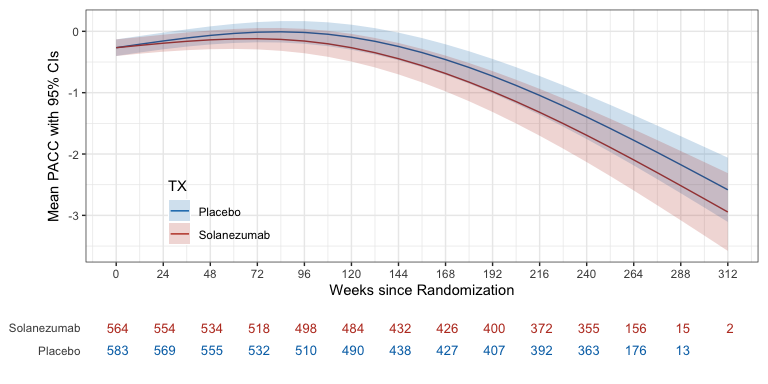
Mean PACC per treatment group over time as estimated by spline model. Shaded region depicts 95% confidence intervals.
Primary analyis of the CFI
# Filter A4LEARN::ADQS for CFITOTAL collected in the blinded phases among mITT population
ADQS_CFI <- A4LEARN::ADQS %>%
  dplyr::filter(MITTFL== 1) %>%
  dplyr::filter(EPOCH == "BLINDED TREATMENT" | AVISIT == "001") %>%
  dplyr::filter(QSTESTCD == "CFITOTAL") %>%
  select(BID, ASEQNCS, TX, ADURW, TX, AGEYR,
    AAPOEGNPRSNFLG, EDCCNTU, SUVRCER, QSSTRESN) %>%
  mutate(TX = factor(TX, levels = c("Placebo", "Solanezumab"))) %>%
  arrange(BID, ADURW) %>%
  na.omit()
ggplot(ADQS_CFI, aes(x=ADURW, y=QSSTRESN, color=TX)) +
  geom_line(aes(group = BID), alpha=0.2) +
  theme(legend.position = "inside", legend.position.inside = c(0.2, 0.9)) +
  xlab("Weeks since Randomization") +
  ylab("CFI Participant and Partner")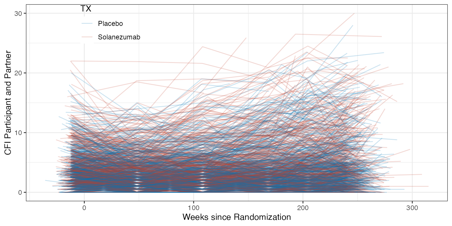
Spaghetti plot of CFI data over time by treatment group.
  scale_x_continuous(breaks = seq(0, max(ADQS_CFI$ADURW), by = 24))
<ScaleContinuousPosition>
 Range:
 Limits:    0 --    1
# Spline basis expansion functions
# CAUTION: these function depend on the ADQS_CFI data frame object in the
# global environment. If ADQS_CFI changes, so do these funtions
ns21 <- function(t){
  as.numeric(predict(splines::ns(ADQS_CFI$ADURW, df=2,
    Boundary.knots = c(0, max(ADQS_CFI$ADURW))), t)[,1])
}
ns22 <- function(t){
  as.numeric(predict(splines::ns(ADQS_CFI$ADURW, df=2,
    Boundary.knots = c(0, max(ADQS_CFI$ADURW))), t)[,2])
}

assign("ns21", ns21, envir = .GlobalEnv)
assign("ns22", ns22, envir = .GlobalEnv)

# GLS model fit:
cfi_fit <- gls(QSSTRESN ~
    I(ns21(ADURW)) + I(ns22(ADURW)) +
    (I(ns21(ADURW)) + I(ns22(ADURW))):TX +
    AGEYR + AAPOEGNPRSNFLG + EDCCNTU + SUVRCER,
  data = ADQS_CFI,
  weights = varIdent(form = ~ 1 | ASEQNCS),
  correlation = corARMA(form = ~ ASEQNCS | BID, p = 5))
ref_grid(cfi_fit,
  at = list(ADURW = c(0,240), TX = levels(ADQS_CFI$TX)),
  vcov. = clubSandwich::vcovCR(cfi_fit, type = "CR2") %>% as.matrix(),
  data = ADQS_CFI,
  mode = "satterthwaite") %>%
  emmeans(~ ADURW | TX) %>%
  pairs(reverse = TRUE) %>%
  as_tibble() %>%
  mutate(p.value = formatp(p.value)) %>%
  kable(caption = "Mean CFI change from baseline at week 240 by treatment
    group estimated from spline model.", digits = 2, booktabs = TRUE) %>%
kableExtra::kable_styling(latex_options = "HOLD_position")| contrast | TX | estimate | SE | df | t.ratio | p.value |
|---|---|---|---|---|---|---|
| ADURW240 - ADURW0 | Placebo | 1.51 | 0.19 | 1845.32 | 7.96 | p<0.001 |
| ADURW240 - ADURW0 | Solanezumab | 2.09 | 0.21 | 2299.16 | 9.77 | p<0.001 |
contrast240 <- ref_grid(cfi_fit,
  at = list(ADURW = 240, TX = levels(ADQS_CFI$TX)),
  vcov. = clubSandwich::vcovCR(cfi_fit, type = "CR2") %>% as.matrix(),
  data = ADQS_CFI,
  mode = "satterthwaite") %>%
  emmeans(specs = "TX", by = "ADURW") %>%
  pairs(reverse = TRUE, adjust = "none")

contrast240 %>%
  as_tibble() %>%
  left_join(contrast240 %>%
      confint() %>%
      as_tibble() %>%
      select(contrast, lower.CL, upper.CL), by="contrast") %>%
  relocate(p.value, .after = last_col()) %>%
  mutate(p.value = formatp(p.value)) %>%
  kable(caption = "Mean CFI group change from baseline at week 240 by treatment
    group estimated from spline model.", digits = 2, booktabs = TRUE) %>%
kableExtra::kable_styling(latex_options = "HOLD_position")| contrast | ADURW | estimate | SE | df | t.ratio | lower.CL | upper.CL | p.value |
|---|---|---|---|---|---|---|---|---|
| Solanezumab - Placebo | 240 | 0.58 | 0.29 | 2103.74 | 2.04 | 0.02 | 1.14 | 0.04 |
ref_grid(cfi_fit,
  at = list(ADURW = seq(0, 312, by=12), TX = levels(ADQS_CFI$TX)),
  vcov. = clubSandwich::vcovCR(cfi_fit, type = "CR2") %>% as.matrix(),
  data = ADQS_CFI,
  mode = "satterthwaite") %>%
  emmeans(specs = "TX", by = "ADURW") %>%
  as_tibble() %>%
  ggplot(aes(x=ADURW, y=emmean)) +
  geom_line(aes(color=TX)) +
  geom_ribbon(aes(ymin = lower.CL, ymax = upper.CL, fill = TX), alpha = 0.2) +
  scale_x_continuous(breaks = seq(0, 312, by=24)) +
  ylab("Mean CFI with 95% confidence intervals") +
  xlab("Weeks since Randomization") +
  theme(legend.position = 'inside', legend.position.inside = c(0.2, 0.9))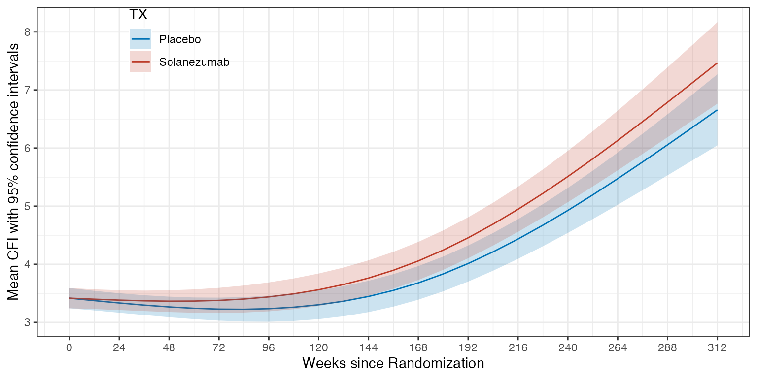
Mean CFI per treatment group over time as estimated by spline model. Shaded region depicts 95% confidence intervals.