NACCADRC Basic Summaries

2026-04-27

Code

library(NACCADRC)
library(ggplot2)
library(tidyverse)
library(nlme)
library(data.table)
library(gtsummary)
library(UpSetR)
library(patchwork)
library(sva)

data(mrisbm, taupetnpdka, phc_cognition, amyloidpetgaain, 
uds_ftldlbd, clariti_edc, uds_mri)

# Data print function
datatable <- function(data, paging = FALSE, searchable = TRUE, bInfo = FALSE, ...) {
  DT::datatable(
    data = data, ...,
    options = list(paging = paging, searchable = searchable, bInfo = bInfo, ...))
}

theme_set(theme_minimal())

scale_colour_discrete <-
  function(...) ggsci::scale_color_jama()
scale_fill_discrete <-
  function(...) ggsci::scale_fill_jama()

cohort_color <- c(CLARiTI = "#C02126", SCAN = "#173058", "Mixed protocol" = "#42B540FF", "SCAN MP" = "#42B540FF")

Merge key imaging and PHC cognitive data

Code

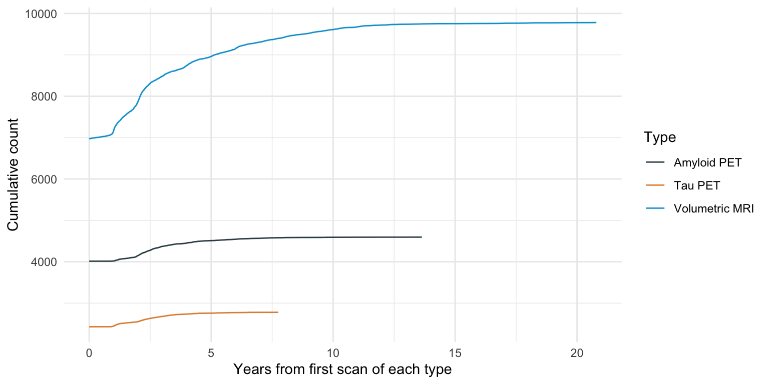
## Combine hippocampal volume from SCAN and Mixed Protocol (UDS) ----
mri_hipp <- mrisbm %>%          # SCAN volumes
  select(SOURCE, NACCID, DATE = SCANDT, HIPPOCAMPUS, ICV = CEREBRUMTCV) %>%
  bind_rows(uds_mri %>%         # Mixed Protocol (UDS) volumes
    select(NACCID, MRIYR, MRIMO, MRIDY, HIPPOCAMPUS = HIPPOVOL, ICV = NACCICV) %>%
    filter(HIPPOCAMPUS != 88.8888, ICV != 9999.999, !is.na(HIPPOCAMPUS)) %>%
    mutate(
      DATE = as.IDate(paste(MRIYR, MRIMO, MRIDY, sep='-')),
      SOURCE = 'Mixed protocol')) %>%
  distinct(NACCID, DATE, .keep_all = TRUE)

NACCETPR_levels <- names(rev(sort(table(uds_ftldlbd$NACCETPR))))

## Combine hipp volume, tau PET, amyloid PET, cognition, and demographics ----
dd_atn <- clariti_edc %>% 
  select(NACCID) %>% distinct() %>% mutate(`CLARiTI EDC` = 'Yes') %>%
  full_join(mri_hipp %>%                 # Hippocampal volumes
      select(NACCID, MRI_SOURCE = SOURCE, DATE, HIPPOCAMPUS, ICV),
    by = 'NACCID') %>%
  full_join(taupetnpdka %>%
      arrange(NACCID, SCANDATE, desc(PROCESSDATE)) %>%
      distinct(NACCID, SCANDATE, .keep_all = TRUE) %>%
      select(NACCID, DATE = SCANDATE, Tau_PET = META_TEMPORAL_SUVR, 
        CTX_ENTORHINAL_SUVR, Tau_TRACER = TRACER, Tau_SOURCE = SOURCE) %>%
      distinct(NACCID, DATE, .keep_all = TRUE),
    by = c('NACCID', 'DATE')) %>%
  full_join(amyloidpetgaain %>%          # Amyloid PET
      arrange(NACCID, SCANDATE, desc(PROCESSDATE)) %>%
      distinct(NACCID, SCANDATE, .keep_all = TRUE) %>%
      select(NACCID, DATE = SCANDATE, AMYLOID_STATUS, CENTILOIDS, 
        Amyloid_TRACER = TRACER, Amyloid_SOURCE = SOURCE) %>%
      distinct(NACCID, DATE, .keep_all = TRUE),
    by = c('NACCID', 'DATE')) %>%
  full_join(phc_cognition %>%            # Harmonized cognition
      select(NACCID, NACCVNUM, PHC_MEM, PHC_EXF, PHC_LAN) %>%
      distinct(NACCID, NACCVNUM, .keep_all = TRUE) %>%
      left_join(uds_ftldlbd %>%          # UDS visit dates
          select(NACCID, NACCVNUM, DATE = VISITDATE),
        by = c('NACCID', 'NACCVNUM')) %>%
      distinct(NACCID, DATE, .keep_all = TRUE),
    by = c('NACCID', 'DATE')) 

stopifnot(with(dd_atn, !any(duplicated(paste(NACCID, DATE)))))

dd <- dd_atn %>%
  full_join(uds_ftldlbd %>%              # UDS diagnosis, etiology over time
      filter(NACCID %in% c(dd_atn$NACCID, clariti_edc$NACCID)) %>%
      mutate(
        NACCETPR = factor(NACCETPR, levels = NACCETPR_levels)) %>%
      select(NACCID, DATE = VISITDATE, NACCUDSD, NACCETPR, PARK) %>%
      distinct(NACCID, DATE, .keep_all = TRUE),
    by = c('NACCID', 'DATE')) %>%
  left_join(uds_ftldlbd %>%              # UDS demographics
      mutate(BIRTHDATE = as.IDate(paste(BIRTHYR, BIRTHMO, 15, sep = '-'))) %>%
      filter(!is.na(BIRTHDATE)) %>%
      arrange(NACCID, NACCVNUM) %>%
      select(NACCID, BIRTHDATE, RACE, SEX = NACCSEX, EDUC, HISPANIC = NACCHISP) %>%
      group_by(NACCID) %>%               # Carry information back/forward
      tidyr::fill(.direction = "updown") %>% # to impute missing data
      ungroup() %>%
      filter(!duplicated(NACCID)),       # One row of demographics per NACCID
    by = 'NACCID') %>%
  arrange(NACCID, DATE) %>%
  group_by(NACCID) %>%                   # Carry Dx information forward/back
  tidyr::fill(all_of(c("NACCUDSD", "NACCETPR", "PARK")), .direction = "downup") %>%
  mutate(ICV = mean(ICV, na.rm = TRUE)) %>% # Average ICV over visits
  ungroup() %>%
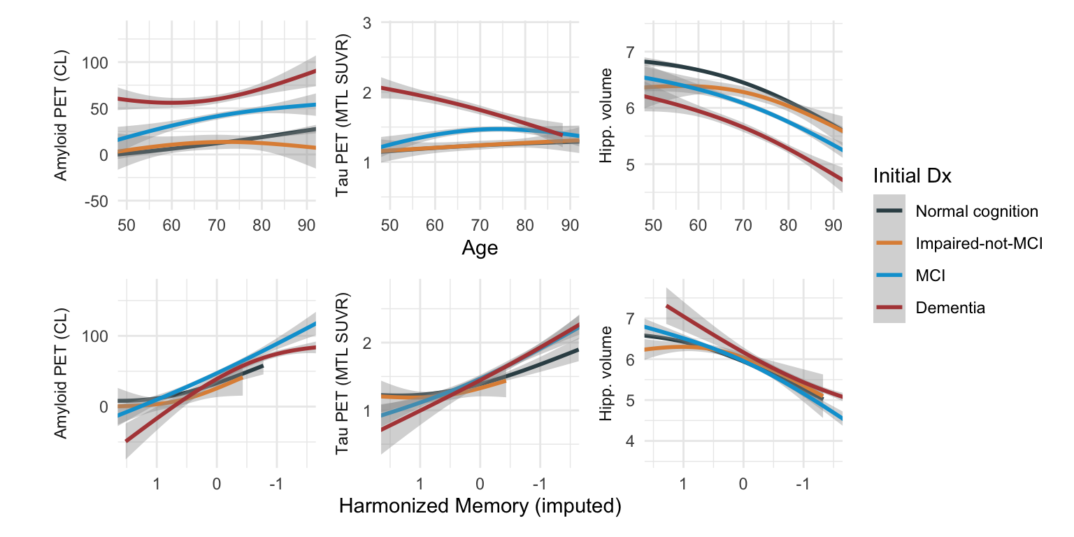
  mutate(
    Age = as.numeric(DATE - BIRTHDATE)/365.25,
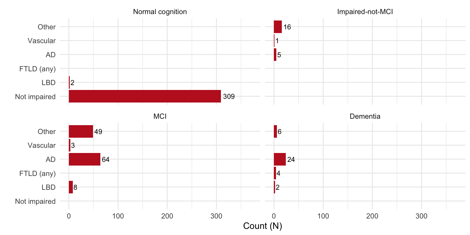
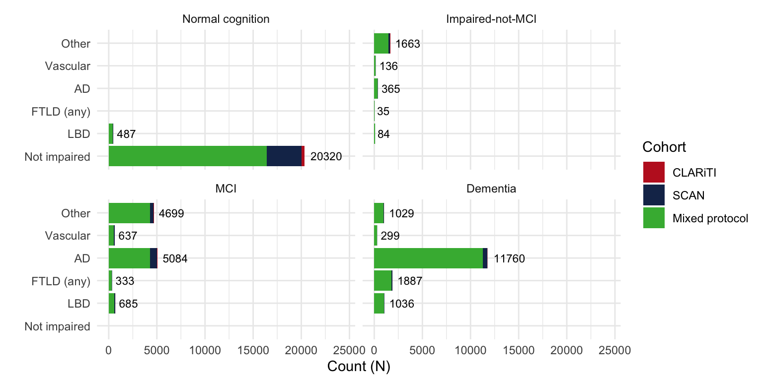
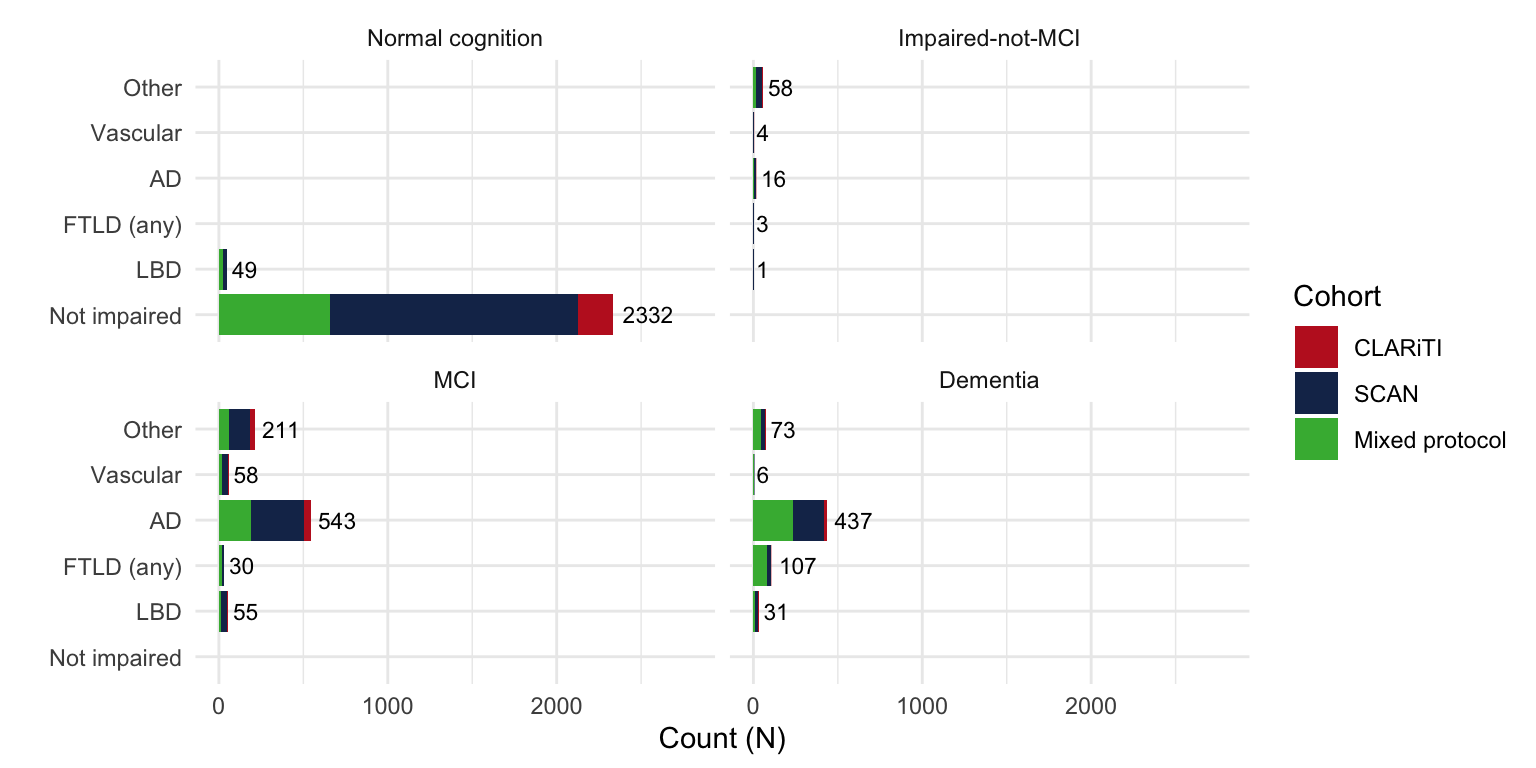
    Etiology = case_when(                     # Simplified/collapse diagnosis
      NACCETPR == "Alzheimer's disease (AD)" ~ 'AD',
      NACCETPR == 'Lewy body disease (LBD)' | PARK == 'Yes' ~ 'LBD',
      NACCETPR %in% c("FTLD, other", "FTLD with motor neuron disease (e.g., ALS)") ~ 
        "FTLD (any)",
      NACCETPR == "Vascular brain injury or vascular dementia including stroke" ~ "Vascular",
      NACCETPR == 'Not applicable, not cognitively impaired' ~ 'Not impaired',
      TRUE ~ 'Other') %>%
      factor(levels = c('Not impaired', 'LBD', "FTLD (any)", 'AD', "Vascular", 'Other')),
    NACCUDSD = case_when(
      is.na(NACCUDSD) ~ 'Unknown',
      TRUE ~ NACCUDSD) %>%
      factor(levels = c("Normal cognition", "Impaired-not-MCI", 
        "MCI", "Dementia", 'Unknown')))

stopifnot(with(dd, !any(duplicated(paste(NACCID, DATE)))))

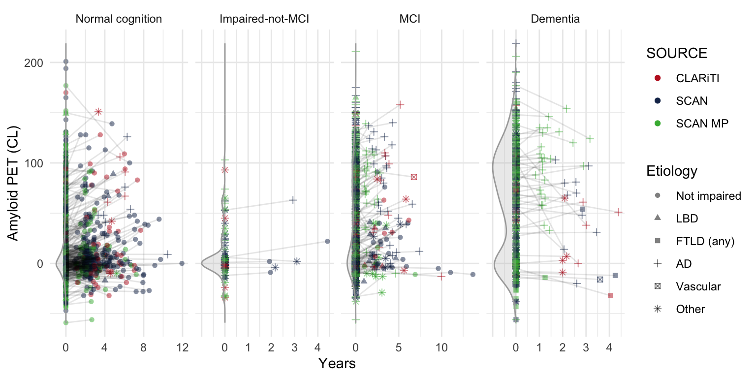
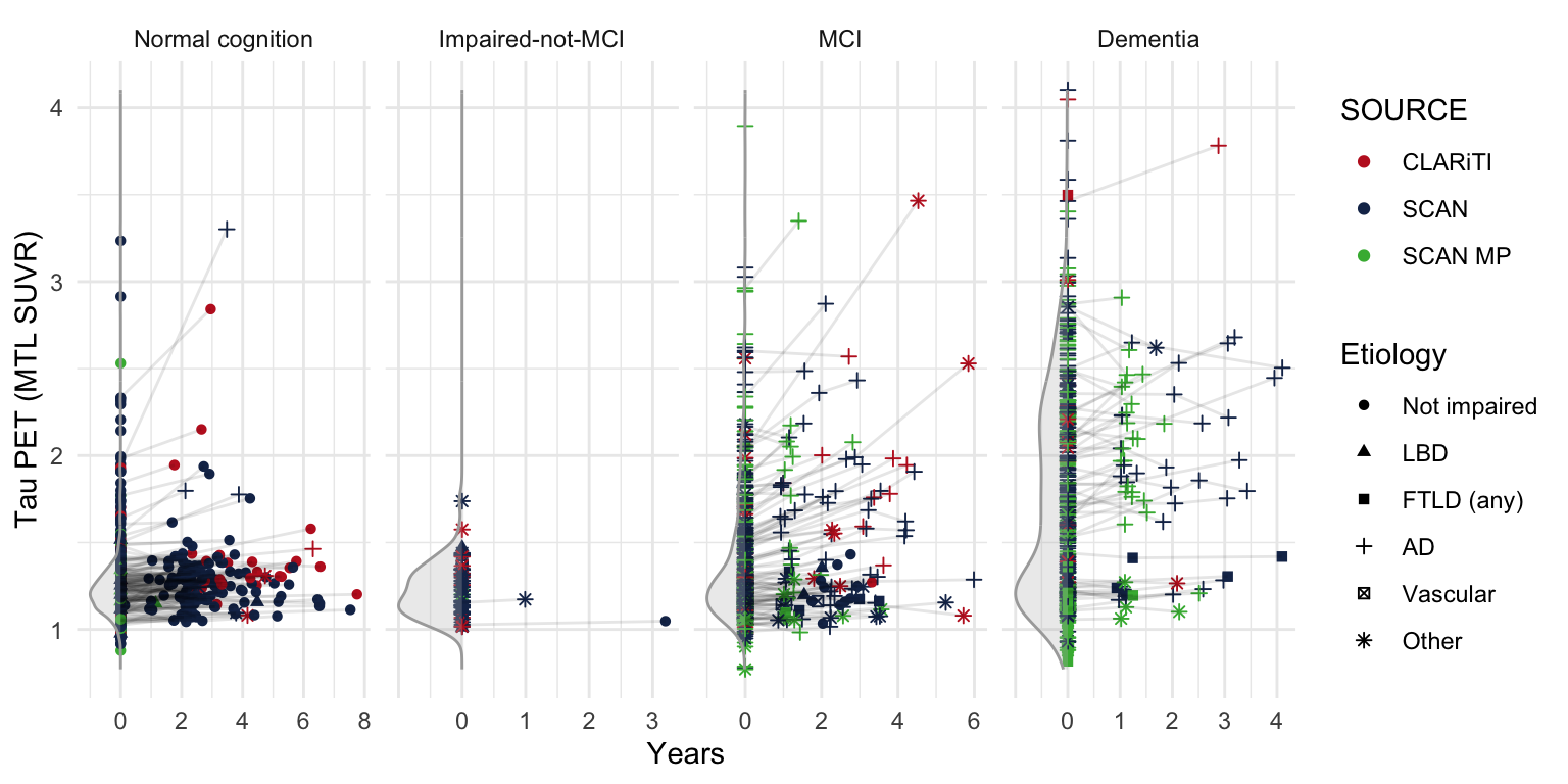
CLARiTI_id <- dd %>%
  filter(MRI_SOURCE == 'CLARiTI' | Tau_SOURCE == 'CLARiTI' | Amyloid_SOURCE == 'CLARiTI') %>%
  pull(NACCID) %>% unique()

SCAN_id <- dd %>%
  filter(MRI_SOURCE == 'SCAN' | Tau_SOURCE == 'SCAN' | Amyloid_SOURCE == 'SCAN') %>%
  pull(NACCID) %>% unique() %>%
  setdiff(CLARiTI_id)

Mixed_id <- setdiff(dd$NACCID, c(CLARiTI_id, SCAN_id))

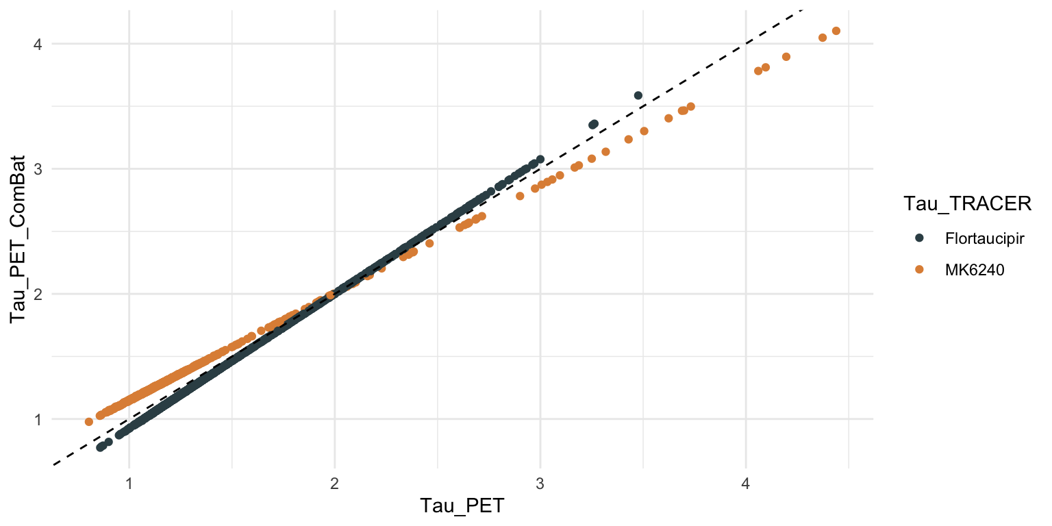
# harmonize tau PET data ----
tmp <- dd %>% filter(!is.na(Tau_PET) & !is.na(Age))
tmp$Tau_PET_ComBat <- sva::ComBat(
  dat=t(tmp[, c('Tau_PET', 'CTX_ENTORHINAL_SUVR')]), 
  batch=tmp$Tau_TRACER, 
  mod=model.matrix(~-1 + Age, tmp), par.prior=TRUE, prior.plots=FALSE)[1,]

dd <- dd %>%
  left_join(tmp %>% select(NACCID, DATE, Tau_PET_ComBat), 
    by = c('NACCID', 'DATE'))

# x-sectional data ----
dd_cross <- dd %>%
  group_by(NACCID) %>%
  fill(everything(), .direction = "updown") %>%
  filter(!duplicated(NACCID)) %>%
  ungroup() %>%
  mutate(    # add labels for tables
    Cohort = case_when(
      NACCID %in% clariti_edc$NACCID ~ 'CLARiTI',
      NACCID %in% CLARiTI_id ~ 'CLARiTI',
      NACCID %in% SCAN_id ~ 'SCAN',
      TRUE ~ 'Mixed protocol') %>%
      factor(levels = c('CLARiTI', 'SCAN', 'Mixed protocol')),
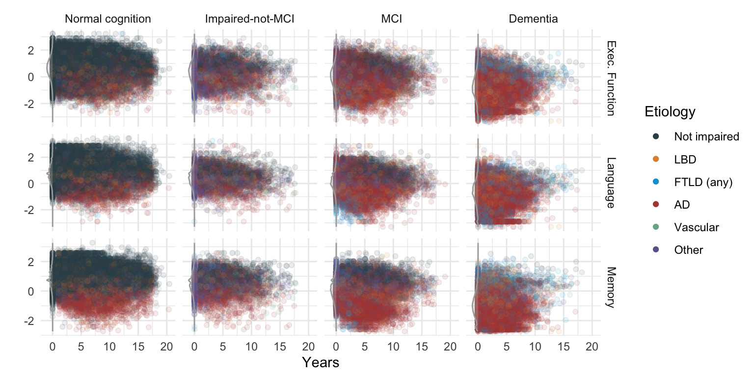
    PHC_MEM = structure(PHC_MEM, label = 'Harmonized Memory'),
    PHC_EXF = structure(PHC_EXF, label = 'Harmonized Exec Function'), 
    PHC_LAN = structure(PHC_LAN, label = 'Harmonized Language'),
    EDUC = structure(EDUC, label = 'Education (yrs)'),
    Age = structure(Age, label = 'Age (yrs)'),
    SEX = structure(SEX, label = 'Sex'),
    RACE = structure(RACE, label = 'Race'),
    HISPANIC = structure(HISPANIC, label = 'Hispanic'),
    AMYLOID_STATUS = structure(AMYLOID_STATUS, label = 'Amyloid status'),
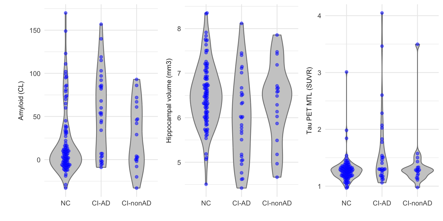
    CENTILOIDS = structure(CENTILOIDS, label = 'Amyloid (CL)'),
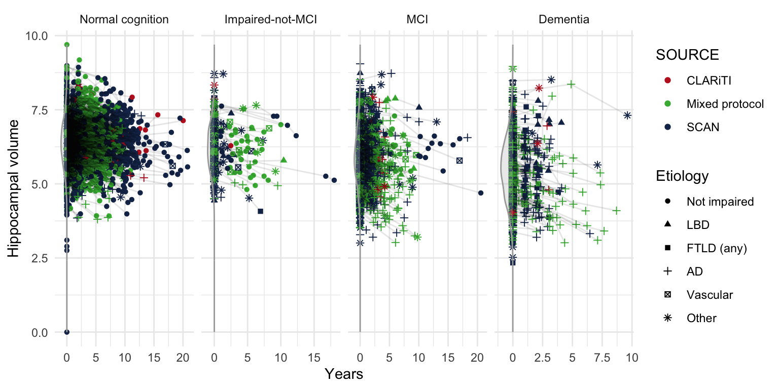
    HIPPOCAMPUS = structure(HIPPOCAMPUS, label = 'Hippocampal volume (mm3)'),
    Tau_PET = structure(Tau_PET, label = 'Tau PET (SUVR)'),
    Tau_PET_ComBat = structure(Tau_PET_ComBat, label = 'Tau PET (SUVR)'),
    Tau_TRACER = structure(Tau_TRACER, label = 'Tau PET tracer'),
    NACCETPR = structure(NACCETPR, label = 'Primary etiologic diagnosis'),
    NACCUDSD = structure(NACCUDSD, label = 'Cognitive status at UDS visit'))

Summarize data collection

CLARiTI imaging distributions

Code

dd_cross %>%
  filter(Cohort == 'CLARiTI') %>%
  filter(NACCUDSD != 'Unknown') %>%
  mutate(
    Diagnosis = case_when(
      NACCUDSD == "Normal cognition" ~ "NC",
      NACCETPR == "Alzheimer's disease (AD)" ~ "CI-AD",
      TRUE ~ "CI-nonAD") %>% factor(c("NC", "CI-AD", "CI-nonAD"))) %>%
  filter(!is.na(Diagnosis), !is.na(CENTILOIDS), !is.na(Tau_PET_ComBat),
    !is.na(HIPPOCAMPUS)) %>%
  select(NACCID, Diagnosis, 
    `Amyloid (CL)` = CENTILOIDS, 
    `Tau PET MTL (SUVR)` = Tau_PET_ComBat, 
    `Hippocampal volume (mm3)` = HIPPOCAMPUS) %>%
  pivot_longer(`Amyloid (CL)`:`Hippocampal volume (mm3)`, 
    names_to = 'Measure', values_to = 'Value') %>%
ggplot(aes(x = Diagnosis, y = Value)) +
  geom_violin(fill = "gray80", color = "gray50") +
  ggbeeswarm::geom_beeswarm(color = "blue", alpha = 0.5) +
  facet_wrap(vars(Measure), nrow = 1, scales = 'free', strip.position = "left") +
  labs(x = "", y = "") +
  theme(legend.position = "none", strip.placement = "outside")

Figure 1: Distribution of imaging summaries among CLARiTI participants with known UDS cognitive status, amyloid PET (CL), hippocampal volume (mm$^3$), and tau PET (SUVR). Tau PET is shown as SUVR harmonized across tracers by ComBat.

Bar charts

Code

plot_data <- dd_cross %>% 
  filter(Cohort == 'CLARiTI') %>%
  filter(NACCUDSD != 'Unknown') %>%
  mutate(across(where(is.factor), fct_drop)) %>%
  group_by(NACCUDSD, Etiology) %>%
  summarise(n = n(), .groups = "drop")
ggplot(plot_data, aes(x = n, y = Etiology)) +
  geom_bar(stat = "identity", fill = cohort_color["CLARiTI"]) +
  geom_text(aes(label = n), hjust = -0.2, size = 3) +
  expand_limits(x = max(plot_data$n) * 1.2) +
  facet_wrap(vars(NACCUDSD)) +
  labs(y = "", x = "Count (N)")

Figure 2: Number of CLARiTI pariticpants by etiology and UDS clinical diagnosis.

Code

count_data <- dd_cross %>% 
  filter(NACCUDSD != 'Unknown') %>%
  mutate(across(where(is.factor), fct_drop)) %>%
  group_by(NACCUDSD, Etiology) %>%
  summarise(n = n(), .groups = "drop")

dd_cross %>% 
  filter(NACCUDSD != 'Unknown') %>%
  mutate(across(where(is.factor), fct_drop)) %>%
  group_by(NACCUDSD, Etiology, Cohort) %>%
  summarise(n = n(), .groups = "drop") %>%
ggplot(aes(x = n, y = Etiology)) +
  geom_bar(aes(fill = Cohort), stat = "identity") +
  geom_text(data = count_data, aes(label = n), 
    hjust = -0.2, size = 3) +
  expand_limits(x = max(count_data$n) * 1.2) +
  facet_wrap(vars(NACCUDSD)) +
  labs(y = "", x = "Count (N)") +
  scale_fill_manual(values = cohort_color)

Figure 3: Number of pariticpants including CLARiTI, SCAN, and mixed-protocol by etiology and UDS clinical diagnosis.

Code

count_data <- dd_cross %>% 
  filter(NACCUDSD != 'Unknown' & !is.na(CENTILOIDS)) %>%
  mutate(across(where(is.factor), fct_drop)) %>%
  group_by(NACCUDSD, Etiology) %>%
  summarise(n = n(), .groups = "drop")

dd_cross %>% 
  filter(NACCUDSD != 'Unknown' & !is.na(CENTILOIDS)) %>%
  mutate(across(where(is.factor), fct_drop)) %>%
  group_by(NACCUDSD, Etiology, Cohort) %>%
  summarise(n = n(), .groups = "drop") %>%
ggplot(aes(x = n, y = Etiology)) +
  geom_bar(aes(fill = Cohort), stat = "identity") +
  geom_text(data = count_data, aes(label = n), 
    hjust = -0.2, size = 3) +
  expand_limits(x = max(count_data$n) * 1.2) +
  facet_wrap(vars(NACCUDSD)) +
  labs(y = "", x = "Count (N)") +
  scale_fill_manual(values = cohort_color)

Figure 4: Number of pariticpants with amyloid PET, including CLARiTI, SCAN, and mixed-protocol by etiology and UDS clinical diagnosis.

Code

count_data <- dd_cross %>% 
  filter(NACCUDSD != 'Unknown' & !is.na(Tau_PET)) %>%
  mutate(across(where(is.factor), fct_drop)) %>%
  group_by(NACCUDSD, Etiology) %>%
  summarise(n = n(), .groups = "drop")

dd_cross %>% 
  filter(NACCUDSD != 'Unknown' & !is.na(Tau_PET)) %>%
  mutate(across(where(is.factor), fct_drop)) %>%
  group_by(NACCUDSD, Etiology, Cohort) %>%
  summarise(n = n(), .groups = "drop") %>%
ggplot(aes(x = n, y = Etiology)) +
  geom_bar(aes(fill = Cohort), stat = "identity") +
  geom_text(data = count_data, aes(label = n), 
    hjust = -0.2, size = 3) +
  expand_limits(x = max(count_data$n) * 1.2) +
  facet_wrap(vars(NACCUDSD)) +
  labs(y = "", x = "Count (N)") +
  scale_fill_manual(values = cohort_color)

Figure 5: Number of pariticpants with tau PET, including CLARiTI, SCAN, and mixed-protocol by etiology and UDS clinical diagnosis.

UpSet plots

Code

dd_upset <- dd_cross %>%
  mutate(
    `CLARiTI EDC` = case_when(`CLARiTI EDC` == 'Yes' ~ 1, TRUE ~ 0),
    Diagnosis = case_when(!is.na(NACCUDSD) &  NACCUDSD != "Unknown" ~ 1, TRUE ~ 0),
    MRI = case_when(!is.na(HIPPOCAMPUS) ~ 1, TRUE ~ 0),
    `Amyloid PET` = case_when(!is.na(CENTILOIDS) ~ 1, TRUE ~ 0),
    `Tau PET` = case_when(!is.na(Tau_PET) ~ 1, TRUE ~ 0)) %>%
  select(NACCID, Cohort, `CLARiTI EDC`, Diagnosis:`Tau PET`) %>%
  as.data.frame()

# Output list CLARiTI participants with missing data for QC ----
if(FALSE){
  qc_dir <- file.path('..', 'reports', 'qc')
  dir.create(qc_dir, recursive = TRUE)
  dd_upset %>% 
    rowwise() %>%
    filter(`CLARiTI EDC` == 1, sum(c_across(MRI:`Tau PET`)) == 0) %>%
    write.csv(file.path(qc_dir, "clariti_edc_no_imaging_participants.csv"), row.names = FALSE)
  
  dd_upset %>% 
    rowwise() %>%
    filter(`CLARiTI EDC` == 1, sum(c_across(Diagnosis:`Tau PET`)) == 0) %>%
    write.csv(file.path(qc_dir, "clariti_edc_only_participants.csv"), row.names = FALSE)
  
  dd_upset %>% 
    filter(Cohort == 'CLARiTI') %>%
    write.csv(file.path(qc_dir, "clariti_participants.csv"), row.names = FALSE)
}

# UpSet plot of CLARiTI participants ----
upset(subset(dd_upset, Cohort == 'CLARiTI'), nsets = 7, nintersects = 30, mb.ratio = c(0.5, 0.5),
  order.by = c("freq", "degree"), decreasing = c(TRUE,FALSE))

Figure 6: UpSet plot of CLARiTI participants.

Code

upset(subset(dd_upset, Cohort %in% c('CLARiTI', 'SCAN')), 
  nsets = 7, nintersects = 30, mb.ratio = c(0.5, 0.5),
  order.by = c("freq", "degree"), decreasing = c(TRUE,FALSE))

Figure 7: UpSet plot of CLARiTI and SCAN participants.

Code

upset(dd_upset, nsets = 7, nintersects = 30, mb.ratio = c(0.5, 0.5),
  order.by = c("freq", "degree"), decreasing = c(TRUE,FALSE))

Figure 8: UpSet plot of all participants.

Scan counts

Code

tmp <- dd %>% 
  select(NACCID, CENTILOIDS, HIPPOCAMPUS, Tau_PET_ComBat) %>%
  rename(
    `Amyloid PET` = CENTILOIDS, `Volumetric MRI` = HIPPOCAMPUS, 
    `Tau PET` = Tau_PET_ComBat) %>%
  group_by(NACCID) %>%
  pivot_longer(`Amyloid PET`:`Tau PET`) %>%
  filter(!is.na(value)) %>%
  mutate(Type = factor(name, levels = c(
    "Amyloid PET", "Tau PET", "Volumetric MRI"))) %>%
  group_by(Type, NACCID) %>%
  summarise(`Serial scans` = n())

with(tmp, table(Type, `Serial scans`)) %>% 
  knitr::kable(caption = "Number of individuals who have received the given number serial scans for each scan type.")

Table 1: Number of individuals who have received the given number serial scans for each scan type.

	1	2	3	4	5	6	7	9
Amyloid PET	3665	494	40	7	0	0	0	0
Tau PET	2107	293	27	2	0	0	0	0
Volumetric MRI	5175	1310	470	122	27	18	3	1

Cummulative scans by time from first scan

Code

dd %>% 
  select(NACCID, Age, Etiology, NACCUDSD, NACCETPR,
    CENTILOIDS, HIPPOCAMPUS, Tau_PET_ComBat) %>%
  rename(
    `Amyloid PET` = CENTILOIDS, `Volumetric MRI` = HIPPOCAMPUS, 
    `Tau PET` = Tau_PET_ComBat) %>%
  pivot_longer(`Amyloid PET`:`Tau PET`) %>%
  filter(!is.na(value), !is.na(Age), !is.na(NACCUDSD)) %>%
  mutate(Type = factor(name, levels = c(
    "Amyloid PET", "Tau PET", "Volumetric MRI"))) %>%
  group_by(NACCID, Type) %>%
  mutate(
    Age0 = min(Age, na.rm = TRUE),
    `Initial Dx` = case_when(
      Age == Age0 ~ NACCUDSD,
      TRUE ~ NA),
    Years = Age - Age0) %>%
  arrange(NACCID, Years) %>%
  tidyr::fill(all_of("Initial Dx"), .direction = "down") %>%
  group_by(Type, Years) %>%
  summarise(count = n()) %>%
  mutate(`Cumulative count` = cumsum(count)) %>%
ggplot(aes(x=Years, y=`Cumulative count`, color = Type)) +
  geom_line() +
  xlab('Years from first scan of each type')

Figure 9: Cumulative scans by time from first scan of each scan type.

Baseline characteristics

CLARiTI participants

Code

tbl_summary(
  data = dd_cross %>% filter(Cohort == 'CLARiTI') %>%
    mutate(across(where(is.factor), fct_drop)),
  by = NACCUDSD,
  include = c("CLARiTI EDC", "Etiology", "Age", "SEX", "EDUC", "RACE", "HISPANIC", "AMYLOID_STATUS", "CENTILOIDS", "HIPPOCAMPUS", "Tau_PET", "Tau_TRACER", "PHC_MEM", "PHC_EXF", "PHC_LAN"),
  type = all_continuous() ~ "continuous2",
  statistic = list(
    all_continuous() ~ c(
      "{mean} ({sd})",
      "{median} ({p25}, {p75})",
      "{min}, {max}"),
    all_categorical() ~ "{n} ({p}%)"),
  digits = all_continuous() ~ 1,
  percent = "row",
  missing_text = "(Missing)") %>%
  add_overall(last = TRUE) %>%
  add_stat_label(label = all_continuous2() ~ c("Mean (SD)", "Median (Q1, Q3)", "Range")) %>%
  modify_caption(caption = "Characteristics of CLARiTI participants by baseline UDS diagnosis. Note CLARiTI participants are those with a NACCID in clariti_edc or any of the CLARiTI imaging summary files.") %>%
  modify_footnote_header(
    footnote = "Row-wise percentage; n (%)",
    columns = all_stat_cols(),
    replace = TRUE) %>%
  bold_labels()

Table 2: Characteristics of CLARiTI participants by baseline UDS diagnosis. Note CLARiTI participants are those with a NACCID in clariti_edc or any of the CLARiTI imaging summary files.

Characteristic	Normal cognition N = 3111	Impaired-not-MCI N = 221	MCI N = 1241	Dementia N = 361	Unknown N = 651	Overall N = 5581
CLARiTI EDC, n (%)
Yes	304 (55%)	22 (4.0%)	124 (23%)	35 (6.4%)	65 (12%)	550 (100%)
(Missing)	7	0	0	1	0	8
Etiology, n (%)
Not impaired	309 (100%)	0 (0%)	0 (0%)	0 (0%)	0 (0%)	309 (100%)
LBD	2 (17%)	0 (0%)	8 (67%)	2 (17%)	0 (0%)	12 (100%)
FTLD (any)	0 (0%)	0 (0%)	0 (0%)	4 (100%)	0 (0%)	4 (100%)
AD	0 (0%)	5 (5.4%)	64 (69%)	24 (26%)	0 (0%)	93 (100%)
Vascular	0 (0%)	1 (25%)	3 (75%)	0 (0%)	0 (0%)	4 (100%)
Other	0 (0%)	16 (12%)	49 (36%)	6 (4.4%)	65 (48%)	136 (100%)
Age (yrs)
Mean (SD)	67.6 (7.0)	68.8 (6.6)	69.7 (7.5)	71.3 (10.0)	NA (NA)	68.4 (7.5)
Median (Q1, Q3)	67.8 (63.1, 72.5)	70.0 (62.9, 73.5)	69.9 (64.5, 74.7)	70.2 (63.8, 80.5)	NA (NA, NA)	68.6 (63.6, 73.2)
Range	43.2, 89.3	55.4, 77.7	49.8, 87.0	52.4, 89.3	Inf, -Inf	43.2, 89.3
(Missing)	0	0	0	0	65	65
Sex, n (%)
Male	101 (50%)	13 (6.5%)	69 (34%)	18 (9.0%)	0 (0%)	201 (100%)
Female	210 (72%)	9 (3.1%)	55 (19%)	18 (6.2%)	0 (0%)	292 (100%)
(Missing)	0	0	0	0	65	65
Education (yrs)
Mean (SD)	16.6 (2.4)	15.7 (3.1)	16.2 (3.0)	16.2 (2.8)	NA (NA)	16.4 (2.6)
Median (Q1, Q3)	16.0 (16.0, 18.0)	16.0 (14.0, 18.0)	16.0 (14.0, 18.0)	16.0 (14.0, 18.0)	NA (NA, NA)	16.0 (15.0, 18.0)
Range	11.0, 25.0	9.0, 20.0	5.0, 22.0	11.0, 20.0	Inf, -Inf	5.0, 25.0
(Missing)	1	0	1	0	65	67
Race, n (%)
White	217 (63%)	11 (3.2%)	87 (25%)	30 (8.7%)	0 (0%)	345 (100%)
Black or African American	56 (61%)	10 (11%)	24 (26%)	2 (2.2%)	0 (0%)	92 (100%)
American Indian or Alaska Native	5 (83%)	0 (0%)	1 (17%)	0 (0%)	0 (0%)	6 (100%)
Asian	13 (81%)	0 (0%)	2 (13%)	1 (6.3%)	0 (0%)	16 (100%)
Other (specify)	3 (75%)	0 (0%)	1 (25%)	0 (0%)	0 (0%)	4 (100%)
Unknown	2 (67%)	0 (0%)	1 (33%)	0 (0%)	0 (0%)	3 (100%)
(Missing)	15	1	8	3	65	92
Hispanic, n (%)
No	277 (63%)	18 (4.1%)	111 (25%)	34 (7.7%)	0 (0%)	440 (100%)
Yes	33 (65%)	3 (5.9%)	13 (25%)	2 (3.9%)	0 (0%)	51 (100%)
Unknown	1 (50%)	1 (50%)	0 (0%)	0 (0%)	0 (0%)	2 (100%)
(Missing)	0	0	0	0	65	65
Amyloid status, n (%)
Negative	122 (65%)	9 (4.8%)	42 (22%)	8 (4.2%)	8 (4.2%)	189 (100%)
Positive	86 (58%)	3 (2.0%)	37 (25%)	16 (11%)	7 (4.7%)	149 (100%)
(Missing)	103	10	45	12	50	220
Amyloid (CL)
Mean (SD)	20.5 (38.6)	7.3 (36.5)	29.8 (37.6)	52.0 (47.5)	20.3 (30.8)	24.5 (39.5)
Median (Q1, Q3)	7.0 (-6.0, 37.5)	0.0 (-14.0, 22.5)	10.0 (-1.0, 60.0)	54.0 (4.0, 77.0)	11.0 (-3.0, 36.0)	8.0 (-3.0, 50.0)
Range	-39.0, 177.0	-34.0, 93.0	-20.0, 140.0	-20.0, 157.0	-8.0, 101.0	-39.0, 177.0
(Missing)	103	10	45	12	50	220
Hippocampal volume (mm3)
Mean (SD)	6.6 (0.7)	6.6 (0.9)	6.1 (0.8)	6.0 (1.2)	6.6 (0.6)	6.4 (0.8)
Median (Q1, Q3)	6.5 (6.1, 7.0)	6.6 (6.1, 7.4)	6.1 (5.5, 6.7)	6.4 (5.2, 6.7)	6.4 (6.1, 7.2)	6.5 (5.9, 7.0)
Range	4.5, 8.4	5.1, 7.9	4.6, 7.9	4.0, 8.1	5.4, 7.5	4.0, 8.4
(Missing)	132	14	61	19	49	275
Tau PET (SUVR)
Mean (SD)	1.2 (0.3)	1.2 (0.2)	1.4 (0.4)	2.1 (1.1)	1.2 (0.1)	1.3 (0.4)
Median (Q1, Q3)	1.2 (1.1, 1.3)	1.2 (1.1, 1.3)	1.3 (1.2, 1.5)	2.0 (1.2, 2.4)	1.2 (1.2, 1.2)	1.2 (1.1, 1.3)
Range	0.9, 3.2	0.8, 1.5	1.0, 2.7	1.0, 4.4	0.9, 1.3	0.8, 4.4
(Missing)	152	12	66	21	58	309
Tau PET tracer, n (%)
Flortaucipir	61 (55%)	3 (2.7%)	32 (29%)	9 (8.2%)	5 (4.5%)	110 (100%)
MK6240	98 (71%)	7 (5.0%)	26 (19%)	6 (4.3%)	2 (1.4%)	139 (100%)
(Missing)	152	12	66	21	58	309
Harmonized Memory
Mean (SD)	1.0 (0.5)	0.5 (0.4)	0.2 (0.6)	-0.2 (0.7)	0.8 (NA)	0.7 (0.6)
Median (Q1, Q3)	0.9 (0.6, 1.3)	0.6 (0.1, 0.9)	0.3 (-0.1, 0.6)	-0.4 (-0.7, 0.4)	0.8 (0.8, 0.8)	0.7 (0.4, 1.1)
Range	-0.3, 2.7	-0.1, 1.0	-1.5, 1.5	-1.2, 1.6	0.8, 0.8	-1.5, 2.7
(Missing)	71	11	43	17	64	206
Harmonized Exec Function
Mean (SD)	0.8 (0.6)	-0.1 (0.6)	0.2 (0.7)	-0.3 (0.7)	0.1 (NA)	0.6 (0.7)
Median (Q1, Q3)	0.8 (0.4, 1.2)	0.1 (-0.4, 0.2)	0.1 (-0.2, 0.7)	-0.3 (-0.8, 0.1)	0.1 (0.1, 0.1)	0.6 (0.1, 1.1)
Range	-1.1, 2.4	-1.3, 0.7	-1.4, 1.9	-1.4, 1.0	0.1, 0.1	-1.4, 2.4
(Missing)	71	11	43	17	64	206
Harmonized Language
Mean (SD)	1.0 (0.6)	0.3 (0.5)	0.4 (0.5)	-0.1 (0.6)	1.7 (NA)	0.8 (0.7)
Median (Q1, Q3)	1.0 (0.6, 1.4)	0.1 (0.0, 0.6)	0.4 (0.0, 0.8)	0.1 (-0.6, 0.3)	1.7 (1.7, 1.7)	0.8 (0.3, 1.2)
Range	-0.4, 2.7	-0.6, 1.3	-1.0, 1.4	-1.0, 0.7	1.7, 1.7	-1.0, 2.7
(Missing)	71	11	43	17	64	206
1 Row-wise percentage; n (%)

All participants

Code

tbl_summary(
  data = dd_cross %>%
    mutate(across(where(is.factor), fct_drop)),
  by = NACCUDSD,
  include = c("Etiology", "Age", "SEX", "EDUC", "RACE", "HISPANIC", "AMYLOID_STATUS", "CENTILOIDS", "HIPPOCAMPUS", "Tau_PET", "Tau_TRACER", "PHC_MEM", "PHC_EXF", "PHC_LAN"),
  type = all_continuous() ~ "continuous2",
  statistic = list(all_continuous() ~ c(
    "{mean} ({sd})",
    "{median} ({p25}, {p75})",
    "{min}, {max}"),
    all_categorical() ~ "{n} ({p}%)"),
  digits = all_continuous() ~ 1,
  percent = "row",
  missing_text = "(Missing)") %>%
  add_overall(last = TRUE) %>%
  add_stat_label(label = all_continuous2() ~ c("Mean (SD)", "Median (Q1, Q3)", "Range")) %>%
  modify_caption(caption = "Characteristics of all participants by baseline UDS diagnosis.") %>%
  modify_footnote_header(
    footnote = "Row-wise percentage; n (%)",
    columns = all_stat_cols(),
    replace = TRUE) %>%
  bold_labels()

Table 3: Characteristics of all participants by baseline UDS diagnosis.

Characteristic	Normal cognition N = 20,8071	Impaired-not-MCI N = 2,2831	MCI N = 11,4381	Dementia N = 16,0111	Unknown N = 5111	Overall N = 51,0501
Etiology, n (%)
Not impaired	20,320 (100%)	0 (0%)	0 (0%)	0 (0%)	0 (0%)	20,320 (100%)
LBD	487 (21%)	84 (3.7%)	685 (30%)	1,036 (45%)	0 (0%)	2,292 (100%)
FTLD (any)	0 (0%)	35 (1.6%)	333 (15%)	1,887 (84%)	0 (0%)	2,255 (100%)
AD	0 (0%)	365 (2.1%)	5,084 (30%)	11,760 (68%)	0 (0%)	17,209 (100%)
Vascular	0 (0%)	136 (13%)	637 (59%)	299 (28%)	0 (0%)	1,072 (100%)
Other	0 (0%)	1,663 (21%)	4,699 (59%)	1,029 (13%)	511 (6.5%)	7,902 (100%)
Age (yrs)
Mean (SD)	70.0 (10.6)	70.0 (10.2)	72.9 (9.2)	72.8 (10.4)	NA (NA)	71.6 (10.3)
Median (Q1, Q3)	70.4 (64.6, 76.8)	70.4 (64.2, 76.8)	73.3 (67.1, 79.1)	74.0 (65.5, 80.5)	NA (NA, NA)	72.1 (65.4, 78.7)
Range	18.0, 104.1	20.2, 102.9	21.8, 109.9	21.9, 104.8	Inf, -Inf	18.0, 109.9
(Missing)	0	0	0	0	511	511
Sex, n (%)
Male	7,150 (33%)	964 (4.5%)	5,680 (26%)	7,756 (36%)	0 (0%)	21,550 (100%)
Female	13,656 (47%)	1,319 (4.6%)	5,757 (20%)	8,255 (28%)	0 (0%)	28,987 (100%)
Prefer not to answer	1 (50%)	0 (0%)	1 (50%)	0 (0%)	0 (0%)	2 (100%)
(Missing)	0	0	0	0	511	511
Education (yrs)
Mean (SD)	15.9 (2.9)	14.8 (3.7)	15.3 (3.4)	14.5 (3.7)	NA (NA)	15.2 (3.4)
Median (Q1, Q3)	16.0 (14.0, 18.0)	16.0 (12.0, 18.0)	16.0 (13.0, 18.0)	15.0 (12.0, 17.0)	NA (NA, NA)	16.0 (13.0, 18.0)
Range	0.0, 29.0	0.0, 24.0	0.0, 31.0	0.0, 30.0	Inf, -Inf	0.0, 31.0
(Missing)	106	9	64	157	511	847
Race, n (%)
White	16,086 (40%)	1,549 (3.9%)	8,861 (22%)	13,396 (34%)	0 (0%)	39,892 (100%)
Black or African American	3,492 (46%)	528 (7.0%)	1,875 (25%)	1,672 (22%)	0 (0%)	7,567 (100%)
American Indian or Alaska Native	210 (43%)	31 (6.4%)	96 (20%)	146 (30%)	0 (0%)	483 (100%)
Native Hawaiian or Other Pacific Islander	18 (33%)	3 (5.6%)	7 (13%)	26 (48%)	0 (0%)	54 (100%)
Asian	594 (47%)	57 (4.5%)	328 (26%)	280 (22%)	0 (0%)	1,259 (100%)
Other (specify)	238 (27%)	90 (10%)	178 (20%)	363 (42%)	0 (0%)	869 (100%)
Unknown	123 (35%)	19 (5.4%)	84 (24%)	124 (35%)	0 (0%)	350 (100%)
(Missing)	46	6	9	4	511	576
Hispanic, n (%)
No	19,012 (41%)	1,968 (4.3%)	10,284 (22%)	14,590 (32%)	0 (0%)	45,854 (100%)
Yes	1,713 (38%)	304 (6.8%)	1,108 (25%)	1,357 (30%)	0 (0%)	4,482 (100%)
Unknown	82 (40%)	11 (5.4%)	46 (23%)	64 (32%)	0 (0%)	203 (100%)
(Missing)	0	0	0	0	511	511
Amyloid status, n (%)
Negative	1,657 (68%)	68 (2.8%)	417 (17%)	192 (7.9%)	107 (4.4%)	2,441 (100%)
Positive	748 (39%)	29 (1.5%)	572 (30%)	490 (25%)	85 (4.4%)	1,924 (100%)
(Missing)	18,402	2,186	10,449	15,329	319	46,685
Amyloid (CL)
Mean (SD)	13.3 (31.1)	12.5 (28.8)	41.2 (47.7)	61.4 (52.7)	25.6 (41.6)	27.2 (43.5)
Median (Q1, Q3)	3.0 (-4.0, 20.0)	2.5 (-4.0, 24.0)	25.0 (0.0, 81.0)	70.0 (6.0, 103.0)	8.0 (-3.0, 43.0)	8.0 (-3.0, 55.0)
Range	-59.0, 201.0	-34.0, 103.0	-56.0, 211.0	-56.0, 219.0	-56.0, 152.0	-59.0, 219.0
(Missing)	18,426	2,201	10,541	15,357	319	46,844
Hippocampal volume (mm3)
Mean (SD)	6.3 (0.8)	6.2 (0.8)	6.0 (0.9)	5.6 (1.0)	6.3 (0.9)	6.2 (0.9)
Median (Q1, Q3)	6.3 (5.8, 6.9)	6.2 (5.6, 6.7)	5.9 (5.3, 6.6)	5.5 (4.9, 6.2)	6.4 (5.7, 6.9)	6.2 (5.6, 6.8)
Range	0.0, 9.7	4.4, 8.7	2.5, 9.1	2.3, 9.0	2.4, 8.2	0.0, 9.7
(Missing)	16,617	1,982	9,826	15,145	354	43,924
Tau PET (SUVR)
Mean (SD)	1.2 (0.2)	1.2 (0.2)	1.4 (0.4)	1.7 (0.6)	1.3 (0.4)	1.4 (0.4)
Median (Q1, Q3)	1.2 (1.1, 1.3)	1.2 (1.1, 1.3)	1.3 (1.2, 1.5)	1.6 (1.2, 2.2)	1.2 (1.1, 1.3)	1.2 (1.2, 1.4)
Range	0.9, 3.4	0.8, 1.9	0.9, 4.2	0.9, 4.4	0.9, 3.7	0.8, 4.4
(Missing)	19,400	2,226	10,884	15,600	336	48,446
Tau PET tracer, n (%)
Flortaucipir	910 (47%)	38 (2.0%)	464 (24%)	396 (20%)	128 (6.6%)	1,936 (100%)
MK6240	504 (73%)	19 (2.8%)	98 (14%)	18 (2.6%)	47 (6.9%)	686 (100%)
(Missing)	19,393	2,226	10,876	15,597	336	48,428
Harmonized Memory
Mean (SD)	0.8 (0.5)	0.4 (0.6)	0.1 (0.6)	-0.9 (0.8)	0.5 (0.9)	0.1 (0.9)
Median (Q1, Q3)	0.7 (0.5, 1.1)	0.4 (0.1, 0.7)	0.1 (-0.3, 0.5)	-0.9 (-1.3, -0.4)	0.7 (-0.2, 1.2)	0.2 (-0.5, 0.7)
Range	-2.4, 2.7	-2.6, 2.4	-2.3, 2.2	-2.7, 2.0	-1.9, 2.0	-2.7, 2.7
(Missing)	805	52	300	213	448	1,818
Harmonized Exec Function
Mean (SD)	0.7 (0.7)	0.2 (0.7)	0.1 (0.7)	-0.7 (0.8)	0.6 (1.0)	0.1 (0.9)
Median (Q1, Q3)	0.7 (0.2, 1.1)	0.3 (-0.2, 0.7)	0.1 (-0.4, 0.5)	-0.7 (-1.2, -0.2)	0.8 (0.2, 1.2)	0.2 (-0.5, 0.7)
Range	-2.7, 3.2	-2.7, 2.7	-3.2, 2.7	-3.3, 2.2	-3.3, 2.2	-3.3, 3.2
(Missing)	783	62	320	1,191	401	2,757
Harmonized Language
Mean (SD)	0.8 (0.6)	0.4 (0.6)	0.2 (0.6)	-0.6 (0.8)	0.8 (0.8)	0.2 (0.9)
Median (Q1, Q3)	0.8 (0.4, 1.2)	0.4 (0.0, 0.8)	0.2 (-0.2, 0.5)	-0.6 (-1.1, -0.1)	0.9 (0.4, 1.3)	0.2 (-0.3, 0.8)
Range	-1.9, 3.3	-2.9, 2.9	-2.9, 2.9	-3.3, 2.9	-1.9, 2.8	-3.3, 3.3
(Missing)	783	61	327	1,158	401	2,730
1 Row-wise percentage; n (%)

Participants with hippocampal volumes

Code

tbl_summary(
  data = dd_cross %>% filter(!is.na(HIPPOCAMPUS)) %>%
    mutate(across(where(is.factor), fct_drop)),
  by = NACCUDSD,
  include = c("Etiology", "Age", "SEX", "EDUC", "RACE", "HISPANIC", "AMYLOID_STATUS", "CENTILOIDS", "HIPPOCAMPUS", "Tau_PET", "Tau_TRACER", "PHC_MEM", "PHC_EXF", "PHC_LAN"),
  type = all_continuous() ~ "continuous2",
  statistic = list(all_continuous() ~ c(
    "{mean} ({sd})",
    "{median} ({p25}, {p75})",
    "{min}, {max}"
  ),
    all_categorical() ~ "{n} ({p}%)"),
  digits = all_continuous() ~ 1,
  percent = "row",
  missing_text = "(Missing)") %>%
  add_overall(last = TRUE) %>%
  add_stat_label(label = all_continuous2() ~ c("Mean (SD)", 
    "Median (Q1, Q3)", "Range")) %>%
  modify_caption(caption = "Characteristics of all participants with MRI data by baseline UDS diagnosis.") %>%
  modify_footnote_header(
    footnote = "Row-wise percentage; n (%)",
    columns = all_stat_cols(),
    replace = TRUE) %>%
  bold_labels()

Table 4: Characteristics of all participants with MRI data by baseline UDS diagnosis.

Characteristic	Normal cognition N = 4,1901	Impaired-not-MCI N = 3011	MCI N = 1,6121	Dementia N = 8661	Unknown N = 1571	Overall N = 7,1261
Etiology, n (%)
Not impaired	4,134 (100%)	0 (0%)	0 (0%)	0 (0%)	0 (0%)	4,134 (100%)
LBD	56 (30%)	8 (4.3%)	84 (45%)	39 (21%)	0 (0%)	187 (100%)
FTLD (any)	0 (0%)	5 (5.6%)	29 (32%)	56 (62%)	0 (0%)	90 (100%)
AD	0 (0%)	36 (2.2%)	887 (55%)	704 (43%)	0 (0%)	1,627 (100%)
Vascular	0 (0%)	32 (18%)	127 (71%)	21 (12%)	0 (0%)	180 (100%)
Other	0 (0%)	220 (24%)	485 (53%)	46 (5.1%)	157 (17%)	908 (100%)
Age (yrs)
Mean (SD)	68.5 (8.9)	68.9 (8.5)	72.2 (8.2)	72.0 (9.4)	NA (NA)	69.8 (9.0)
Median (Q1, Q3)	69.0 (63.4, 74.3)	68.6 (63.8, 75.3)	72.4 (66.6, 77.8)	73.1 (65.9, 79.0)	NA (NA, NA)	70.2 (64.4, 75.9)
Range	21.3, 100.1	36.4, 92.0	27.7, 98.7	30.2, 94.2	Inf, -Inf	21.3, 100.1
(Missing)	0	0	0	0	157	157
Sex, n (%)
Male	1,426 (51%)	128 (4.5%)	836 (30%)	431 (15%)	0 (0%)	2,821 (100%)
Female	2,763 (67%)	173 (4.2%)	776 (19%)	435 (10%)	0 (0%)	4,147 (100%)
Prefer not to answer	1 (100%)	0 (0%)	0 (0%)	0 (0%)	0 (0%)	1 (100%)
(Missing)	0	0	0	0	157	157
Education (yrs)
Mean (SD)	16.1 (2.8)	14.8 (3.8)	15.5 (3.3)	15.2 (3.5)	NA (NA)	15.8 (3.1)
Median (Q1, Q3)	16.0 (14.0, 18.0)	16.0 (12.0, 18.0)	16.0 (13.0, 18.0)	16.0 (12.0, 18.0)	NA (NA, NA)	16.0 (14.0, 18.0)
Range	0.0, 25.0	0.0, 24.0	0.0, 31.0	0.0, 25.0	Inf, -Inf	0.0, 31.0
(Missing)	12	1	5	2	157	177
Race, n (%)
White	3,178 (59%)	190 (3.6%)	1,216 (23%)	766 (14%)	0 (0%)	5,350 (100%)
Black or African American	769 (62%)	85 (6.9%)	311 (25%)	74 (6.0%)	0 (0%)	1,239 (100%)
American Indian or Alaska Native	64 (77%)	4 (4.8%)	15 (18%)	0 (0%)	0 (0%)	83 (100%)
Native Hawaiian or Other Pacific Islander	3 (100%)	0 (0%)	0 (0%)	0 (0%)	0 (0%)	3 (100%)
Asian	94 (59%)	8 (5.1%)	43 (27%)	13 (8.2%)	0 (0%)	158 (100%)
Other (specify)	45 (61%)	5 (6.8%)	16 (22%)	8 (11%)	0 (0%)	74 (100%)
Unknown	26 (63%)	4 (9.8%)	8 (20%)	3 (7.3%)	0 (0%)	41 (100%)
(Missing)	11	5	3	2	157	178
Hispanic, n (%)
No	3,770 (60%)	256 (4.1%)	1,462 (23%)	785 (13%)	0 (0%)	6,273 (100%)
Yes	407 (61%)	44 (6.6%)	140 (21%)	78 (12%)	0 (0%)	669 (100%)
Unknown	13 (48%)	1 (3.7%)	10 (37%)	3 (11%)	0 (0%)	27 (100%)
(Missing)	0	0	0	0	157	157
Amyloid status, n (%)
Negative	921 (78%)	33 (2.8%)	174 (15%)	33 (2.8%)	25 (2.1%)	1,186 (100%)
Positive	424 (54%)	12 (1.5%)	235 (30%)	97 (12%)	16 (2.0%)	784 (100%)
(Missing)	2,845	256	1,203	736	116	5,156
Amyloid (CL)
Mean (SD)	13.1 (31.1)	10.3 (29.2)	39.4 (46.8)	62.3 (52.4)	18.0 (36.1)	21.7 (39.5)
Median (Q1, Q3)	3.0 (-4.0, 19.0)	2.0 (-5.0, 18.0)	23.5 (-1.0, 74.0)	63.0 (12.5, 101.0)	8.0 (-3.0, 27.0)	6.0 (-4.0, 38.0)
Range	-42.0, 201.0	-34.0, 93.0	-40.0, 175.0	-22.0, 219.0	-56.0, 110.0	-56.0, 219.0
(Missing)	2,849	258	1,218	738	116	5,179
Hippocampal volume (mm3)
Mean (SD)	6.3 (0.8)	6.2 (0.8)	6.0 (0.9)	5.6 (1.0)	6.3 (0.9)	6.2 (0.9)
Median (Q1, Q3)	6.3 (5.8, 6.9)	6.2 (5.6, 6.7)	5.9 (5.3, 6.6)	5.5 (4.9, 6.2)	6.4 (5.7, 6.9)	6.2 (5.6, 6.8)
Range	0.0, 9.7	4.4, 8.7	2.5, 9.1	2.3, 9.0	2.4, 8.2	0.0, 9.7
Tau PET (SUVR)
Mean (SD)	1.2 (0.2)	1.2 (0.2)	1.4 (0.4)	1.9 (0.7)	1.3 (0.4)	1.3 (0.4)
Median (Q1, Q3)	1.2 (1.1, 1.3)	1.2 (1.1, 1.3)	1.3 (1.2, 1.5)	1.8 (1.3, 2.2)	1.2 (1.2, 1.3)	1.2 (1.1, 1.3)
Range	0.9, 3.4	0.8, 1.9	0.9, 3.3	1.0, 4.4	1.0, 3.7	0.8, 4.4
(Missing)	3,283	269	1,325	746	109	5,732
Tau PET tracer, n (%)
Flortaucipir	498 (56%)	18 (2.0%)	213 (24%)	108 (12%)	46 (5.2%)	883 (100%)
MK6240	411 (80%)	14 (2.7%)	75 (15%)	13 (2.5%)	2 (0.4%)	515 (100%)
(Missing)	3,281	269	1,324	745	109	5,728
Harmonized Memory
Mean (SD)	0.9 (0.5)	0.5 (0.6)	0.1 (0.6)	-0.8 (0.7)	1.0 (0.3)	0.5 (0.8)
Median (Q1, Q3)	0.8 (0.5, 1.2)	0.5 (0.1, 0.9)	0.1 (-0.3, 0.5)	-0.8 (-1.2, -0.4)	1.0 (0.8, 1.4)	0.6 (0.0, 1.0)
Range	-0.9, 2.6	-0.8, 2.2	-1.8, 2.0	-2.7, 1.5	0.5, 1.5	-2.7, 2.6
(Missing)	514	35	182	76	149	956
Harmonized Exec Function
Mean (SD)	0.7 (0.7)	0.2 (0.8)	0.1 (0.6)	-0.6 (0.8)	0.6 (0.5)	0.4 (0.8)
Median (Q1, Q3)	0.7 (0.3, 1.2)	0.3 (-0.3, 0.8)	0.1 (-0.3, 0.5)	-0.6 (-1.2, -0.1)	0.6 (0.3, 1.0)	0.4 (-0.1, 1.0)
Range	-1.8, 3.2	-2.2, 2.2	-2.3, 2.7	-3.3, 1.9	-0.3, 1.2	-3.3, 3.2
(Missing)	514	36	185	88	149	972
Harmonized Language
Mean (SD)	0.9 (0.6)	0.5 (0.6)	0.2 (0.6)	-0.5 (0.7)	1.0 (0.6)	0.5 (0.8)
Median (Q1, Q3)	0.8 (0.5, 1.3)	0.4 (0.1, 0.8)	0.2 (-0.1, 0.6)	-0.4 (-0.9, 0.0)	0.9 (0.6, 1.0)	0.6 (0.1, 1.1)
Range	-1.2, 3.3	-1.2, 2.3	-1.9, 2.6	-2.9, 1.5	0.2, 2.4	-2.9, 3.3
(Missing)	514	36	184	86	149	969
1 Row-wise percentage; n (%)

Participants with tau PET

Code

tbl_summary(
  data = dd_cross %>% filter(!is.na(Tau_PET)) %>%
    mutate(across(where(is.factor), fct_drop)),
  by = NACCUDSD,
  include = c("Etiology", "Age", "SEX", "EDUC", "RACE", "HISPANIC", "AMYLOID_STATUS", "CENTILOIDS", "HIPPOCAMPUS", "Tau_PET", "Tau_TRACER", "PHC_MEM", "PHC_EXF", "PHC_LAN"),
  type = all_continuous() ~ "continuous2",
  statistic = list(all_continuous() ~ c(
    "{mean} ({sd})",
    "{median} ({p25}, {p75})",
    "{min}, {max}"),
    all_categorical() ~ "{n} ({p}%)"),
  digits = all_continuous() ~ 1,
  percent = "row",
  missing_text = "(Missing)") %>%
  add_overall(last = TRUE) %>%
  add_stat_label(label = all_continuous2() ~ c("Mean (SD)", "Median (Q1, Q3)", "Range")) %>%
  modify_caption(caption = "Characteristics of all participants with tau PET data by baseline UDS diagnosis.") %>%
  modify_footnote_header(
    footnote = "Row-wise percentage; n (%)",
    columns = all_stat_cols(),
    replace = TRUE) %>%
  bold_labels()

Table 5: Characteristics of all participants with tau PET data by baseline UDS diagnosis.

Characteristic	Normal cognition N = 1,4071	Impaired-not-MCI N = 571	MCI N = 5541	Dementia N = 4111	Unknown N = 1751	Overall N = 2,6041
Etiology, n (%)
Not impaired	1,395 (100%)	0 (0%)	0 (0%)	0 (0%)	0 (0%)	1,395 (100%)
LBD	12 (30%)	2 (5.0%)	17 (43%)	9 (23%)	0 (0%)	40 (100%)
FTLD (any)	0 (0%)	2 (2.0%)	27 (26%)	73 (72%)	0 (0%)	102 (100%)
AD	0 (0%)	11 (1.8%)	325 (54%)	269 (44%)	0 (0%)	605 (100%)
Vascular	0 (0%)	3 (6.8%)	39 (89%)	2 (4.5%)	0 (0%)	44 (100%)
Other	0 (0%)	39 (9.3%)	146 (35%)	58 (14%)	175 (42%)	418 (100%)
Age (yrs)
Mean (SD)	67.2 (8.6)	67.4 (8.4)	69.4 (8.3)	67.9 (10.0)	NA (NA)	67.9 (8.8)
Median (Q1, Q3)	67.9 (62.3, 73.1)	67.1 (62.9, 73.4)	70.1 (64.3, 75.0)	68.0 (61.0, 75.8)	NA (NA, NA)	68.4 (62.5, 74.0)
Range	22.2, 92.2	36.4, 80.9	27.3, 95.5	22.5, 87.6	Inf, -Inf	22.2, 95.5
(Missing)	0	0	0	0	175	175
Sex, n (%)
Male	498 (49%)	32 (3.2%)	281 (28%)	202 (20%)	0 (0%)	1,013 (100%)
Female	909 (64%)	25 (1.8%)	273 (19%)	209 (15%)	0 (0%)	1,416 (100%)
(Missing)	0	0	0	0	175	175
Education (yrs)
Mean (SD)	16.4 (2.4)	15.9 (2.6)	16.2 (2.8)	16.0 (3.0)	NA (NA)	16.3 (2.6)
Median (Q1, Q3)	16.0 (15.0, 18.0)	16.0 (14.0, 18.0)	16.0 (14.0, 18.0)	16.0 (14.0, 18.0)	NA (NA, NA)	16.0 (14.0, 18.0)
Range	8.0, 25.0	11.0, 23.0	8.0, 26.0	3.0, 30.0	Inf, -Inf	3.0, 30.0
(Missing)	2	0	5	6	175	188
Race, n (%)
White	1,031 (54%)	36 (1.9%)	456 (24%)	372 (20%)	0 (0%)	1,895 (100%)
Black or African American	285 (73%)	14 (3.6%)	71 (18%)	20 (5.1%)	0 (0%)	390 (100%)
American Indian or Alaska Native	35 (80%)	3 (6.8%)	5 (11%)	1 (2.3%)	0 (0%)	44 (100%)
Native Hawaiian or Other Pacific Islander	2 (50%)	0 (0%)	2 (50%)	0 (0%)	0 (0%)	4 (100%)
Asian	20 (59%)	1 (2.9%)	10 (29%)	3 (8.8%)	0 (0%)	34 (100%)
Other (specify)	6 (43%)	1 (7.1%)	1 (7.1%)	6 (43%)	0 (0%)	14 (100%)
Unknown	5 (28%)	0 (0%)	5 (28%)	8 (44%)	0 (0%)	18 (100%)
(Missing)	23	2	4	1	175	205
Hispanic, n (%)
No	1,305 (57%)	53 (2.3%)	524 (23%)	390 (17%)	0 (0%)	2,272 (100%)
Yes	96 (66%)	4 (2.7%)	28 (19%)	18 (12%)	0 (0%)	146 (100%)
Unknown	6 (55%)	0 (0%)	2 (18%)	3 (27%)	0 (0%)	11 (100%)
(Missing)	0	0	0	0	175	175
Amyloid status, n (%)
Negative	664 (64%)	30 (2.9%)	194 (19%)	86 (8.3%)	57 (5.5%)	1,031 (100%)
Positive	297 (39%)	8 (1.1%)	227 (30%)	179 (24%)	42 (5.6%)	753 (100%)
(Missing)	446	19	133	146	76	820
Amyloid (CL)
Mean (SD)	13.6 (30.2)	8.8 (27.6)	35.5 (45.2)	56.0 (51.3)	27.8 (43.7)	25.8 (41.6)
Median (Q1, Q3)	3.0 (-3.0, 18.0)	-1.0 (-4.0, 8.0)	17.0 (-2.0, 74.0)	63.0 (3.0, 100.0)	5.0 (-3.0, 46.0)	6.0 (-2.0, 50.0)
Range	-59.0, 170.0	-33.0, 93.0	-56.0, 171.0	-56.0, 191.0	-36.0, 138.0	-59.0, 191.0
(Missing)	446	19	133	146	76	820
Hippocampal volume (mm3)
Mean (SD)	6.4 (0.8)	6.3 (0.8)	6.0 (0.9)	5.6 (1.1)	6.4 (0.8)	6.3 (0.9)
Median (Q1, Q3)	6.4 (5.9, 6.9)	6.3 (5.7, 7.0)	6.0 (5.4, 6.7)	5.6 (5.0, 6.3)	6.4 (5.7, 7.1)	6.3 (5.7, 6.9)
Range	3.4, 8.7	4.9, 7.9	3.0, 8.5	2.3, 8.3	4.6, 8.2	2.3, 8.7
(Missing)	500	25	267	291	127	1,210
Tau PET (SUVR)
Mean (SD)	1.2 (0.2)	1.2 (0.2)	1.4 (0.4)	1.7 (0.6)	1.3 (0.4)	1.4 (0.4)
Median (Q1, Q3)	1.2 (1.1, 1.3)	1.2 (1.1, 1.3)	1.3 (1.2, 1.5)	1.6 (1.2, 2.2)	1.2 (1.1, 1.3)	1.2 (1.2, 1.4)
Range	0.9, 3.4	0.8, 1.9	0.9, 4.2	0.9, 4.4	0.9, 3.7	0.8, 4.4
Tau PET tracer, n (%)
Flortaucipir	904 (47%)	38 (2.0%)	456 (24%)	393 (20%)	128 (6.7%)	1,919 (100%)
MK6240	503 (73%)	19 (2.8%)	98 (14%)	18 (2.6%)	47 (6.9%)	685 (100%)
Harmonized Memory
Mean (SD)	0.9 (0.5)	0.6 (0.5)	0.2 (0.5)	-0.5 (0.7)	1.1 (0.3)	0.5 (0.7)
Median (Q1, Q3)	0.9 (0.6, 1.3)	0.5 (0.2, 0.8)	0.3 (-0.1, 0.6)	-0.5 (-1.0, 0.0)	1.0 (0.7, 1.5)	0.6 (0.1, 1.0)
Range	-0.3, 2.7	-0.1, 1.6	-1.3, 2.0	-2.6, 1.5	0.7, 1.5	-2.6, 2.7
(Missing)	307	20	96	92	168	683
Harmonized Exec Function
Mean (SD)	0.8 (0.6)	0.4 (0.5)	0.2 (0.6)	-0.6 (0.9)	0.4 (0.5)	0.4 (0.9)
Median (Q1, Q3)	0.8 (0.4, 1.2)	0.5 (0.1, 0.8)	0.2 (-0.2, 0.6)	-0.6 (-1.2, 0.0)	0.3 (0.0, 0.9)	0.5 (0.0, 1.0)
Range	-1.5, 2.9	-1.1, 1.2	-1.8, 2.0	-3.2, 1.4	-0.3, 1.1	-3.2, 2.9
(Missing)	305	20	96	89	168	678
Harmonized Language
Mean (SD)	0.9 (0.6)	0.6 (0.5)	0.4 (0.6)	-0.4 (0.7)	0.8 (0.4)	0.6 (0.8)
Median (Q1, Q3)	0.9 (0.5, 1.3)	0.6 (0.2, 1.0)	0.4 (0.0, 0.7)	-0.3 (-0.7, 0.2)	0.9 (0.5, 1.2)	0.6 (0.1, 1.1)
Range	-0.9, 2.9	-0.8, 1.3	-1.4, 2.2	-2.5, 1.5	0.2, 1.3	-2.5, 2.9
(Missing)	305	20	96	90	168	679
1 Row-wise percentage; n (%)

Participants with amyloid PET

Code

tbl_summary(
  data = dd_cross %>% filter(!is.na(CENTILOIDS)) %>%
    mutate(across(where(is.factor), fct_drop)),
  by = NACCUDSD,
  include = c("Etiology", "Age", "SEX", "EDUC", "RACE", "HISPANIC", "AMYLOID_STATUS", "CENTILOIDS", "HIPPOCAMPUS", "Tau_PET", "Tau_TRACER", "PHC_MEM", "PHC_EXF", "PHC_LAN"),
  type = all_continuous() ~ "continuous2",
  statistic = list(all_continuous() ~ c(
    "{mean} ({sd})",
    "{median} ({p25}, {p75})",
    "{min}, {max}"
  ),
    all_categorical() ~ "{n} ({p}%)"),
  digits = all_continuous() ~ 1,
  percent = "row",
  missing_text = "(Missing)") %>%
  add_overall(last = TRUE) %>%
  add_stat_label(label = all_continuous2() ~ c("Mean (SD)", "Median (Q1, Q3)", "Range")) %>%
  modify_caption(caption = "Characteristics of NACC ADRC participants with amyloid PET data by baseline UDS diagnosis.") %>%
  modify_footnote_header(
    footnote = "Row-wise percentage; n (%)",
    columns = all_stat_cols(),
    replace = TRUE) %>%
  bold_labels()

Table 6: Characteristics of NACC ADRC participants with amyloid PET data by baseline UDS diagnosis.

Characteristic	Normal cognition N = 2,3811	Impaired-not-MCI N = 821	MCI N = 8971	Dementia N = 6541	Unknown N = 1921	Overall N = 4,2061
Etiology, n (%)
Not impaired	2,332 (100%)	0 (0%)	0 (0%)	0 (0%)	0 (0%)	2,332 (100%)
LBD	49 (36%)	1 (0.7%)	55 (40%)	31 (23%)	0 (0%)	136 (100%)
FTLD (any)	0 (0%)	3 (2.1%)	30 (21%)	107 (76%)	0 (0%)	140 (100%)
AD	0 (0%)	16 (1.6%)	543 (55%)	437 (44%)	0 (0%)	996 (100%)
Vascular	0 (0%)	4 (5.9%)	58 (85%)	6 (8.8%)	0 (0%)	68 (100%)
Other	0 (0%)	58 (11%)	211 (40%)	73 (14%)	192 (36%)	534 (100%)
Age (yrs)
Mean (SD)	68.5 (8.2)	67.3 (8.8)	70.5 (8.3)	67.9 (9.5)	NA (NA)	68.8 (8.5)
Median (Q1, Q3)	68.7 (64.3, 73.7)	68.7 (61.4, 73.2)	70.9 (65.3, 76.5)	67.7 (60.9, 75.4)	NA (NA, NA)	69.2 (64.0, 74.5)
Range	21.3, 93.4	36.9, 83.2	27.3, 95.5	22.5, 90.8	Inf, -Inf	21.3, 95.5
(Missing)	0	0	0	0	192	192
Sex, n (%)
Male	809 (49%)	30 (1.8%)	476 (29%)	349 (21%)	0 (0%)	1,664 (100%)
Female	1,572 (67%)	52 (2.2%)	421 (18%)	305 (13%)	0 (0%)	2,350 (100%)
(Missing)	0	0	0	0	192	192
Education (yrs)
Mean (SD)	16.5 (2.6)	15.6 (2.8)	16.3 (2.8)	15.8 (3.0)	NA (NA)	16.3 (2.7)
Median (Q1, Q3)	16.0 (15.0, 18.0)	16.0 (13.0, 18.0)	16.0 (14.0, 18.0)	16.0 (14.0, 18.0)	NA (NA, NA)	16.0 (14.0, 18.0)
Range	2.0, 25.0	7.0, 20.0	4.0, 26.0	3.0, 30.0	Inf, -Inf	2.0, 30.0
(Missing)	6	0	7	13	192	218
Race, n (%)
White	1,803 (57%)	57 (1.8%)	735 (23%)	574 (18%)	0 (0%)	3,169 (100%)
Black or African American	445 (72%)	18 (2.9%)	113 (18%)	40 (6.5%)	0 (0%)	616 (100%)
American Indian or Alaska Native	43 (75%)	3 (5.3%)	9 (16%)	2 (3.5%)	0 (0%)	57 (100%)
Native Hawaiian or Other Pacific Islander	1 (33%)	0 (0%)	2 (67%)	0 (0%)	0 (0%)	3 (100%)
Asian	55 (57%)	2 (2.1%)	24 (25%)	15 (16%)	0 (0%)	96 (100%)
Other (specify)	12 (52%)	1 (4.3%)	4 (17%)	6 (26%)	0 (0%)	23 (100%)
Unknown	8 (29%)	0 (0%)	5 (18%)	15 (54%)	0 (0%)	28 (100%)
(Missing)	14	1	5	2	192	214
Hispanic, n (%)
No	2,194 (59%)	70 (1.9%)	826 (22%)	619 (17%)	0 (0%)	3,709 (100%)
Yes	179 (63%)	12 (4.2%)	65 (23%)	30 (10%)	0 (0%)	286 (100%)
Unknown	8 (42%)	0 (0%)	6 (32%)	5 (26%)	0 (0%)	19 (100%)
(Missing)	0	0	0	0	192	192
Amyloid status, n (%)
Negative	1,640 (69%)	58 (2.5%)	373 (16%)	187 (7.9%)	107 (4.5%)	2,365 (100%)
Positive	741 (40%)	24 (1.3%)	524 (28%)	467 (25%)	85 (4.6%)	1,841 (100%)
Amyloid (CL)
Mean (SD)	13.3 (31.1)	12.5 (28.8)	41.2 (47.7)	61.4 (52.7)	25.6 (41.6)	27.2 (43.5)
Median (Q1, Q3)	3.0 (-4.0, 20.0)	2.5 (-4.0, 24.0)	25.0 (0.0, 81.0)	70.0 (6.0, 103.0)	8.0 (-3.0, 43.0)	8.0 (-3.0, 55.0)
Range	-59.0, 201.0	-34.0, 103.0	-56.0, 211.0	-56.0, 219.0	-56.0, 152.0	-59.0, 219.0
Hippocampal volume (mm3)
Mean (SD)	6.4 (0.8)	6.2 (0.8)	6.0 (0.9)	5.7 (1.1)	6.3 (0.8)	6.3 (0.9)
Median (Q1, Q3)	6.4 (5.8, 6.9)	6.1 (5.6, 6.8)	5.9 (5.4, 6.7)	5.6 (5.0, 6.5)	6.1 (5.7, 6.9)	6.3 (5.7, 6.9)
Range	3.1, 9.0	4.9, 7.9	2.5, 8.5	2.3, 8.1	5.1, 7.8	2.3, 9.0
(Missing)	1,040	39	503	526	151	2,259
Tau PET (SUVR)
Mean (SD)	1.2 (0.2)	1.2 (0.2)	1.4 (0.4)	1.7 (0.6)	1.3 (0.4)	1.3 (0.4)
Median (Q1, Q3)	1.2 (1.1, 1.3)	1.2 (1.1, 1.3)	1.3 (1.2, 1.5)	1.6 (1.2, 2.2)	1.2 (1.1, 1.3)	1.2 (1.1, 1.3)
Range	0.9, 3.4	0.8, 1.9	0.9, 4.2	0.9, 4.4	0.9, 2.9	0.8, 4.4
(Missing)	1,420	44	476	389	93	2,422
Tau PET tracer, n (%)
Flortaucipir	513 (44%)	22 (1.9%)	332 (28%)	251 (21%)	57 (4.9%)	1,175 (100%)
MK6240	452 (73%)	16 (2.6%)	92 (15%)	17 (2.7%)	42 (6.8%)	619 (100%)
(Missing)	1,416	44	473	386	93	2,412
Harmonized Memory
Mean (SD)	0.9 (0.5)	0.5 (0.5)	0.2 (0.6)	-0.6 (0.7)	1.0 (0.4)	0.5 (0.8)
Median (Q1, Q3)	0.9 (0.6, 1.3)	0.5 (0.2, 0.7)	0.2 (-0.2, 0.6)	-0.6 (-1.0, -0.1)	0.9 (0.8, 1.5)	0.7 (0.1, 1.0)
Range	-0.7, 2.7	-0.7, 1.6	-1.5, 2.0	-2.7, 1.6	0.4, 1.6	-2.7, 2.7
(Missing)	310	17	142	87	182	738
Harmonized Exec Function
Mean (SD)	0.8 (0.6)	0.4 (0.6)	0.2 (0.6)	-0.6 (0.9)	0.3 (0.6)	0.4 (0.8)
Median (Q1, Q3)	0.8 (0.3, 1.2)	0.4 (0.0, 0.9)	0.2 (-0.2, 0.6)	-0.6 (-1.2, 0.0)	0.4 (0.1, 0.8)	0.5 (0.0, 1.0)
Range	-1.5, 2.9	-1.3, 1.6	-1.8, 2.0	-3.2, 2.2	-0.8, 1.1	-3.2, 2.9
(Missing)	308	17	142	92	182	741
Harmonized Language
Mean (SD)	0.9 (0.6)	0.5 (0.5)	0.3 (0.6)	-0.4 (0.7)	0.8 (0.5)	0.6 (0.8)
Median (Q1, Q3)	0.9 (0.5, 1.3)	0.5 (0.1, 0.8)	0.3 (-0.1, 0.7)	-0.3 (-0.9, 0.1)	0.8 (0.5, 1.2)	0.6 (0.1, 1.1)
Range	-0.9, 3.1	-0.8, 1.9	-1.7, 2.3	-2.9, 1.5	0.0, 1.7	-2.9, 3.1
(Missing)	308	17	142	88	182	737
1 Row-wise percentage; n (%)

Summary plots

LOESS Trends

Code

pd1 <- dd %>% 
  select(NACCID, Age, Etiology, NACCUDSD, NACCETPR,
    CENTILOIDS, HIPPOCAMPUS, Tau_PET_ComBat) %>%
  rename(
    `Amyloid PET (CL)` = CENTILOIDS, `Hipp. volume` = HIPPOCAMPUS, 
    `Tau PET (MTL SUVR)` = Tau_PET_ComBat) %>%
  group_by(NACCID) %>%
  mutate(
    Age0 = min(Age),
    `Initial Dx` = case_when(
      Age == Age0 ~ NACCUDSD,
      TRUE ~ NA),
    Years = Age - Age0) %>%
  arrange(NACCID, Years) %>%
  tidyr::fill(all_of("Initial Dx"), .direction = "down") %>%
  pivot_longer(`Amyloid PET (CL)`:`Tau PET (MTL SUVR)`) %>%
  filter(!is.na(value), !is.na(Years), !is.na(NACCUDSD)) %>%
  mutate(name = factor(name, levels = c(
    "Amyloid PET (CL)", "Tau PET (MTL SUVR)", "Hipp. volume")))

pd2_0 <- dd %>% 
  select(NACCID, Age, Memory = PHC_MEM, Etiology, NACCUDSD, NACCETPR,
    CENTILOIDS, HIPPOCAMPUS, Tau_PET_ComBat) %>%
  group_by(NACCID) %>%
  mutate(
    Age0 = min(Age),
    `Initial Dx` = case_when(
      Age == Age0 ~ NACCUDSD,
      TRUE ~ NA),
    Years = Age - Age0) %>%
  arrange(NACCID, Years) %>%
  tidyr::fill(all_of("Initial Dx"), .direction = "down") %>%
  mutate(
    Dx0 = `Initial Dx`,
    Memory_int = zoo::na.approx(Memory, na.rm = FALSE)) %>%
  select(NACCID, Age, `Initial Dx`, Dx0, Memory, Memory_int, Etiology, 
    NACCUDSD, NACCETPR, CENTILOIDS, HIPPOCAMPUS, Tau_PET_ComBat) %>%
  filter(!is.na(Age), !is.na(Dx0)) %>%
  ungroup()

fit_mem <- lme(Memory ~ I(Age^3)*Dx0, 
  random = ~ Age | NACCID, data = pd2_0, na.action = na.omit)
pd2_0$Memory_lme <- predict(fit_mem, newdata = pd2_0 %>% select(-Memory)) %>%
  as.numeric()

pd2 <- pd2_0 %>%
  mutate(
    Memory_i = case_when(
      !is.na(Memory) ~ Memory,
      !is.na(Memory_int) ~ Memory_int,
      !is.na(Memory_lme) ~ Memory_lme)) %>%
  rename(
    `Amyloid PET (CL)` = CENTILOIDS, `Hipp. volume` = HIPPOCAMPUS, 
    `Tau PET (MTL SUVR)` = Tau_PET_ComBat) %>%
  pivot_longer(`Amyloid PET (CL)`:`Tau PET (MTL SUVR)`) %>%
  filter(!is.na(value), !is.na(Memory_i), !is.na(NACCUDSD)) %>%
  mutate(name = factor(name, levels = c(
    "Amyloid PET (CL)", "Tau PET (MTL SUVR)", "Hipp. volume")))

p1 <- ggplot(pd1, aes(x=Age, y=value, color = `Initial Dx`)) +
  facet_wrap(vars(name), scales = 'free_y', ncol = 3, strip.position = "left") +
  geom_smooth(method = 'gam', formula = y ~ s(x, bs = "cs", fx = TRUE, k = 1)) +
  coord_cartesian(xlim = c(50, 90)) +
  ylab('') +
  theme(strip.placement = "outside")

p2 <- ggplot(pd2, aes(x=Memory_i, y=value, color = `Initial Dx`)) +
  facet_wrap(vars(name), scales = 'free_y', ncol = 3, strip.position = "left") +
  geom_smooth(method = 'gam', 
    formula = y ~ s(x, bs = "cs", k = 2, sp = 1)) +
  coord_cartesian(xlim = c(-1.5, 1.5)) +
  ylab('Amyloid PET (CL)') +
  xlab('Harmonized Memory (imputed)') +
  scale_x_reverse() +
  ylab('') +
  theme(strip.placement = "outside")

p1 / p2 + plot_layout(guides = "collect")

LOESS plots. For the bottom plot, memory scores are imputed using linear interpolation (when possible) and a linear mixed effects model (when interpolation was not possible) to allow for plotting against biomarker values. The linear mixed effects model included fixed effects for age (as a cubic polynomial) by initial diagnosis. Random effects included random intercepts and slopes for each participant.

Spaghetti plots

Code

pd <- dd %>% 
  select(NACCID, SOURCE = Amyloid_SOURCE, Etiology, Age, NACCUDSD, NACCETPR, CENTILOIDS) %>%
  filter(!is.na(CENTILOIDS), !is.na(Age)) %>%
  group_by(NACCID) %>%
  mutate(
    Age0 = min(Age),
    `Initial Dx` = case_when(
      Age == Age0 ~ NACCUDSD,
      TRUE ~ NA),
    Years = Age - Age0) %>%
  arrange(NACCID, Years) %>%
  tidyr::fill(all_of("Initial Dx"), .direction = "down")

ggplot(pd, aes(x = Years, y = CENTILOIDS)) +
  geom_point(aes(color = SOURCE, shape = Etiology), alpha = 0.5) +
  geom_line(aes(group = NACCID), alpha=0.1) +
  geom_density(aes(y = CENTILOIDS, 
    x = after_stat(-scaled)), 
    color = "darkgray", fill = "gray", alpha = 0.3, 
    orientation = "y", inherit.aes = FALSE) +
  scale_x_continuous(labels = function(x) ifelse(x < 0, "", x)) +
  facet_grid(. ~ `Initial Dx`, scales = 'free_x') +
  guides(colour = guide_legend(override.aes = list(alpha=1))) +
  ylab('Amyloid PET (CL)') +
  scale_color_manual(values = cohort_color)

Spaghetti plot of amyloid PET.

Code

pd <- dd %>% 
  select(NACCID, SOURCE = Tau_SOURCE, Etiology, Age, NACCUDSD, NACCETPR, Tau_PET_ComBat) %>%
  filter(!is.na(Tau_PET_ComBat), !is.na(Age)) %>%
  group_by(NACCID) %>%
  mutate(
    Age0 = min(Age),
    `Initial Dx` = case_when(
      Age == Age0 ~ NACCUDSD,
      TRUE ~ NA),
    Years = Age - Age0) %>%
  arrange(NACCID, Years) %>%
  tidyr::fill(all_of("Initial Dx"), .direction = "down")

ggplot(pd, aes(x=Years, y=Tau_PET_ComBat)) +
  geom_point(aes(color=SOURCE, shape = Etiology), alpha=1) +
  geom_line(aes(group = NACCID), alpha=0.1) +
  geom_density(aes(y = Tau_PET_ComBat, 
    x = after_stat(-scaled)), 
    color = "darkgray", fill = "gray", alpha = 0.3, 
    orientation = "y", inherit.aes = FALSE) +
  scale_x_continuous(labels = function(x) ifelse(x < 0, "", x)) +
  facet_grid(. ~ `Initial Dx`, scales = 'free_x') +
  guides(colour = guide_legend(override.aes = list(alpha=1))) +
  ylab('Tau PET (MTL SUVR)') +
  scale_color_manual(values = cohort_color)

Spaghetti plot of tau PET.

Code

pd <- dd %>% 
  select(NACCID, SOURCE = MRI_SOURCE, Etiology, Age, NACCUDSD, NACCETPR, HIPPOCAMPUS) %>%
  filter(!is.na(HIPPOCAMPUS), !is.na(Age)) %>%
  group_by(NACCID) %>%
  mutate(
    Age0 = min(Age),
    `Initial Dx` = case_when(
      Age == Age0 ~ NACCUDSD,
      TRUE ~ NA),
    Years = Age - Age0) %>%
  arrange(NACCID, Years) %>%
  tidyr::fill(all_of("Initial Dx"), .direction = "down")

ggplot(pd, aes(x=Years, y=HIPPOCAMPUS)) +
  geom_point(aes(color=SOURCE, shape = Etiology), alpha=1) +
  geom_line(aes(group = NACCID), alpha=0.1) +
  geom_density(aes(y = HIPPOCAMPUS, 
    x = after_stat(-scaled)), 
    color = "darkgray", fill = "gray", alpha = 0.3, 
    orientation = "y", inherit.aes = FALSE) +
  scale_x_continuous(labels = function(x) ifelse(x < 0, "", x)) +
  facet_grid(. ~ `Initial Dx`, scales = 'free_x') +
  guides(colour = guide_legend(override.aes = list(alpha=1))) +
  ylab('Hippocampal volume') +
  scale_color_manual(values = cohort_color)

Spaghetti plot of hippocampal volumes.

Code

pd <- dd %>% 
  select(NACCID, Age, Etiology, NACCUDSD, NACCETPR,
    PHC_MEM, PHC_EXF, PHC_LAN) %>%
  rename(Memory = PHC_MEM, `Exec. Function` = PHC_EXF, Language = PHC_LAN) %>%
  group_by(NACCID) %>%
  mutate(
    Age0 = min(Age),
    `Initial Dx` = case_when(
      Age == Age0 ~ NACCUDSD,
      TRUE ~ NA),
    Years = Age - Age0) %>%
  arrange(NACCID, Years) %>%
  tidyr::fill(all_of("Initial Dx"), .direction = "down") %>%
  pivot_longer(Memory:Language) %>%
  filter(!is.na(value), !is.na(Years), !is.na(NACCUDSD))

ggplot(pd, aes(x=Years, y=value)) +
  geom_point(aes(color = Etiology), alpha=0.1) +
  geom_density(aes(y = value, 
    x = after_stat(-scaled)), 
    color = "darkgray", fill = "gray", alpha = 0.3, 
    orientation = "y", inherit.aes = FALSE) +
  scale_x_continuous(labels = function(x) ifelse(x < 0, "", x)) +
  facet_grid(name ~ `Initial Dx`, scales = 'free_y') +
  guides(colour = guide_legend(override.aes = list(alpha=1))) +
  ylab('')

Spaghetti plot of harmonized cognitive scores.

ComBat Harmonization of tau PET (tracers)

Code

ggplot(dd %>% filter(!is.na(Tau_PET_ComBat)), 
  aes(x = Tau_PET, y = Tau_PET_ComBat, color = Tau_TRACER)) +
  geom_point() +
  geom_abline(intercept = 0, slope = 1, linetype = 'dashed')

ComBat transformed versus raw Tau PET data by tracer.

Publishing with NACC Data

See the author checklist for more information. If you use the NACCADRC R data package, please also cite (Donohue et al. 2026).

Funding

Work on this R package was funded by CLARiTI (NIH U01 AG082350). The NACC database is funded by NIA/NIH Grant U24 AG072122. SCAN was funded by NIA/NIH U24 AG067418. See naccdata.org for more information.

References

Donohue, Michael C, Kedir Hussen, Oliver Langford, Richard Gallardo, Gustavo Jimenez-Maggiora, Paul S Aisen, and Alzheimer’s Disease Neuroimaging Initiative. 2026. “Alzheimer’s clinical research data via R packages: The alzverse.” Alzheimer’s & Dementia 22 (2): e71152. https://doi.org/10.1002/alz.71152.