ADNI-Enrollment
Last Updated: November 12, 2025
Source:vignettes/ADNI-Enrollment.Rmd
ADNI-Enrollment.RmdIntroduction
This article demonstrate how to use the ADNIMERGE2 R
package to generate simple enrollment summaries.
Load Required R Packages
library(tidyverse)
library(gtsummary)
library(labelled)
library(ggplot2)
library(see)
library(ADNIMERGE2)
# Abbreviation list
abbrev_list <- paste0(
  paste0(
    "CN: Cognitive Normal; MCI: Mild Cognitive Impairment; DEM: Dementia; "
  ),
  paste0(
    "SD: Standard Deviation; Q1: the 25th percentile; Q3: the 75th percentile; "
  ),
  paste0(
    "Baseline mPACCdigit score was based on subjects that were ",
    "enrolled only in ADNI1 study phase. "
  ),
  collapse = "\n "
)
conts_statistic_label <- c("Mean (SD)", "Median (Q1, Q3)", "Range")
ADNI Enrollment Summaries
Enrollment Overtime
enroll_summary_data <- ADSL %>%
  filter(ENRLFL %in% "Y") %>%
  mutate(ENRLDT = floor_date(ENRLDT, unit = "month")) %>%
  group_by(ENRLDT, ORIGPROT) %>%
  summarise(num_enroll = n()) %>%
  ungroup() %>%
  mutate(ORIGPROT = factor(ORIGPROT, levels = adni_phase())) %>%
  arrange(ENRLDT, ORIGPROT) %>%
  mutate(cum_num_enroll = cumsum(num_enroll))

enroll_summary_plot <- enroll_summary_data %>%
  ggplot(aes(x = ENRLDT, y = cum_num_enroll, color = ORIGPROT)) +
  geom_line() +
  scale_x_date(
    date_minor_breaks = "2 years",
    limits = range(enroll_summary_data$ENRLDT)
  ) +
  labs(
    x = "Timeline Calendar",
    y = "Cumulative Enrollment Per Month",
    color = "ADNI Study Phase"
  ) +
  theme(axis.text.x = element_text(hjust = 0.3, vjust = 0, angle = 15))
enroll_summary_plot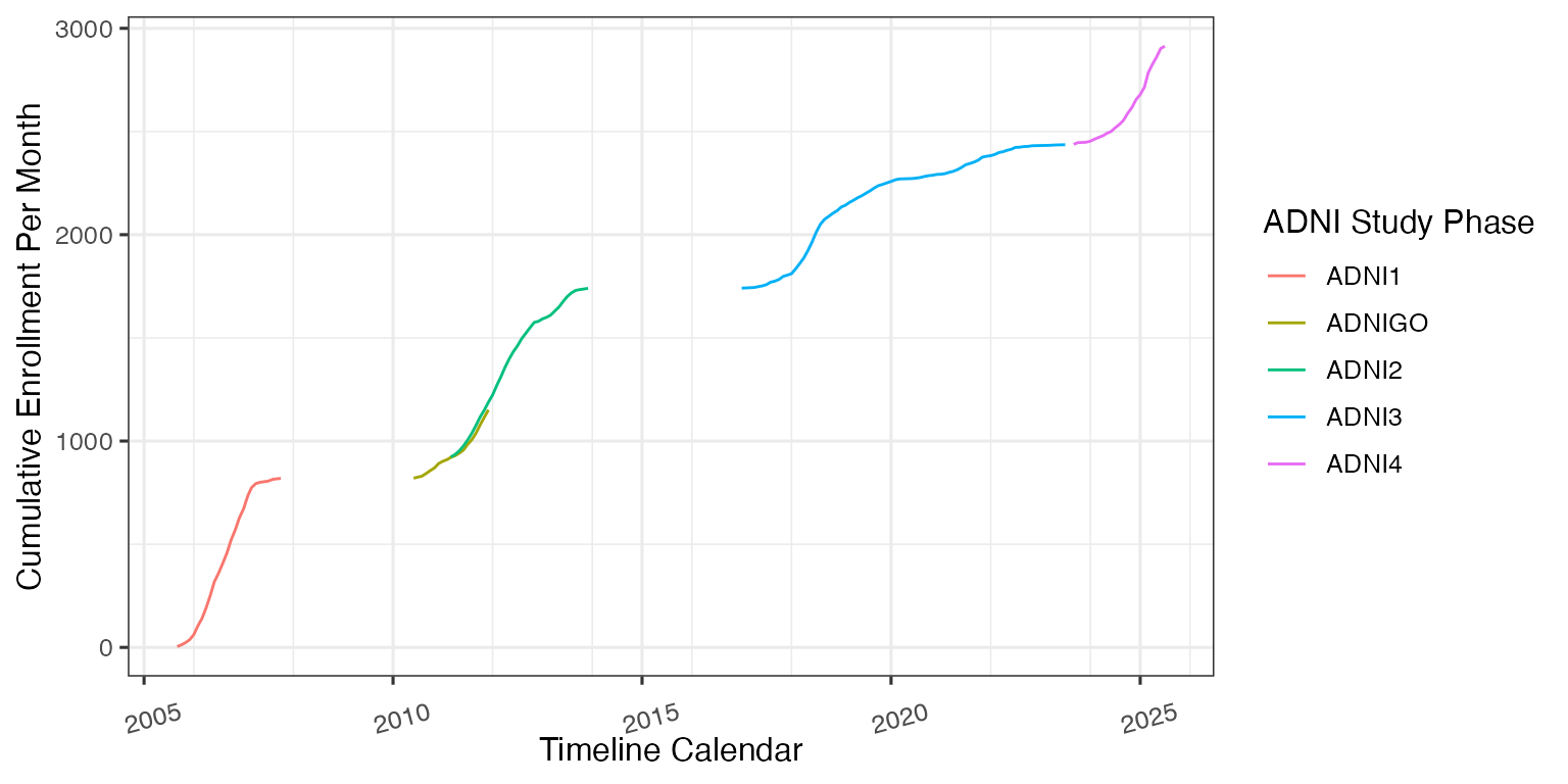
Demographic Summaries: By Study Phase
include_vars <- c(
  "AGE", "SEX", "EDUC", "RACE", "ETHNIC", "MARISTAT",
  "DX", "APOE", "ADASTT13", "CDGLOBAL", "CDRSB", "MMSCORE",
  "FAQTOTAL", "MPACCTRAILSB", "MPACCDIGIT"
)

tbl_summary(
  data = ADSL %>%
    filter(ENRLFL %in% "Y"),
  by = ORIGPROT,
  include = include_vars,
  type = all_continuous() ~ "continuous2",
  statistic = list(
    all_continuous() ~ c(
      "{mean} ({sd})",
      "{median} ({p25}, {p75})",
      "{min}, {max}"
    ),
    all_categorical() ~ "{n} ({p}%)"
  ),
  digits = all_continuous() ~ 1,
  percent = "column",
  missing_text = "(Missing)"
) %>%
  add_overall(last = TRUE) %>%
  add_stat_label(label = all_continuous2() ~ conts_statistic_label) %>%
  modify_footnote_header(
    footnote = "Column-wise percentage; n (%)",
    columns = all_stat_cols(),
    replace = TRUE
  ) %>%
  modify_abbreviation(abbreviation = abbrev_list) %>%
  modify_caption(
    caption = "Table 1. ADNI - Subject Characteristics: By Study Phase"
  ) %>%
bold_labels()| Characteristic |
ADNI1 N = 8191 |
ADNIGO N = 1311 |
ADNI2 N = 7901 |
ADNI3 N = 6961 |
ADNI4 N = 5961 |
Overall N = 3,0321 |
|---|---|---|---|---|---|---|
| Age (in Years) | ||||||
| Mean (SD) | 75.2 (6.8) | 71.6 (7.9) | 72.7 (7.2) | 70.7 (7.4) | 69.1 (7.6) | 72.2 (7.6) |
| Median (Q1, Q3) | 75.6 (71.2, 80.1) | 71.1 (65.8, 77.4) | 72.8 (67.8, 77.6) | 70.0 (65.9, 75.8) | 69.0 (63.0, 74.4) | 72.2 (66.8, 77.6) |
| Range | 54.5, 90.9 | 55.6, 88.3 | 55.0, 91.4 | 50.5, 90.7 | 55.0, 90.8 | 50.5, 91.4 |
| (Missing) | 0 | 0 | 0 | 0 | 1 | 1 |
| Sex, n (%) | ||||||
| Female | 342 (42%) | 60 (46%) | 379 (48%) | 381 (55%) | 367 (62%) | 1,529 (50%) |
| Male | 477 (58%) | 71 (54%) | 411 (52%) | 315 (45%) | 229 (38%) | 1,503 (50%) |
| Education | ||||||
| Mean (SD) | 15.5 (3.0) | 15.8 (2.7) | 16.3 (2.6) | 16.4 (2.3) | 15.8 (2.9) | 16.0 (2.8) |
| Median (Q1, Q3) | 16.0 (13.0, 18.0) | 16.0 (14.0, 18.0) | 16.0 (14.0, 18.0) | 16.0 (15.0, 18.0) | 16.0 (14.0, 18.0) | 16.0 (14.0, 18.0) |
| Range | 4.0, 20.0 | 10.0, 20.0 | 8.0, 20.0 | 10.0, 20.0 | 7.0, 20.0 | 4.0, 20.0 |
| (Missing) | 1 | 0 | 0 | 0 | 2 | 3 |
| Race, n (%) | ||||||
| American Indian or Alaskan Native | 1 (0.1%) | 1 (0.8%) | 1 (0.1%) | 2 (0.3%) | 4 (0.7%) | 9 (0.3%) |
| Asian | 14 (1.7%) | 1 (0.8%) | 14 (1.8%) | 29 (4.2%) | 49 (8.2%) | 107 (3.5%) |
| Black or African American | 39 (4.8%) | 4 (3.1%) | 34 (4.3%) | 105 (15%) | 207 (35%) | 389 (13%) |
| Native Hawaiian or Other Pacific Islander | 0 (0%) | 0 (0%) | 2 (0.3%) | 1 (0.1%) | 2 (0.3%) | 5 (0.2%) |
| Other Pacific Islander | 0 (0%) | 0 (0%) | 0 (0%) | 0 (0%) | 0 (0%) | 0 (0%) |
| White | 762 (93%) | 118 (90%) | 728 (92%) | 537 (77%) | 297 (50%) | 2,442 (81%) |
| More than one race | 3 (0.4%) | 5 (3.8%) | 10 (1.3%) | 13 (1.9%) | 26 (4.4%) | 57 (1.9%) |
| Unknown | 0 (0%) | 2 (1.5%) | 1 (0.1%) | 9 (1.3%) | 11 (1.8%) | 23 (0.8%) |
| Ethnicity, n (%) | ||||||
| Hispanic or Latino | 19 (2.3%) | 8 (6.1%) | 31 (3.9%) | 58 (8.3%) | 78 (13%) | 194 (6.4%) |
| Not Hispanic or Latino | 794 (97%) | 122 (93%) | 755 (96%) | 637 (92%) | 516 (87%) | 2,824 (93%) |
| Unknown | 6 (0.7%) | 1 (0.8%) | 4 (0.5%) | 1 (0.1%) | 2 (0.3%) | 14 (0.5%) |
| Marital Status, n (%) | ||||||
| Divorced | 52 (6.4%) | 17 (13%) | 82 (10%) | 79 (11%) | 107 (18%) | 337 (11%) |
| Domestic Partnership | 0 (0%) | 0 (0%) | 0 (0%) | 0 (0%) | 13 (2.2%) | 13 (0.4%) |
| Married | 629 (77%) | 95 (73%) | 586 (74%) | 517 (74%) | 348 (59%) | 2,175 (72%) |
| Never married | 28 (3.4%) | 3 (2.3%) | 33 (4.2%) | 35 (5.0%) | 76 (13%) | 175 (5.8%) |
| Unknown | 1 (0.1%) | 4 (3.1%) | 2 (0.3%) | 2 (0.3%) | 0 (0%) | 9 (0.3%) |
| Widowed | 108 (13%) | 12 (9.2%) | 87 (11%) | 62 (8.9%) | 50 (8.4%) | 319 (11%) |
| (Missing) | 1 | 0 | 0 | 1 | 2 | 4 |
| Baseline Diagnostics Status, n (%) | ||||||
| CN | 229 (28%) | 1 (0.8%) | 295 (37%) | 378 (54%) | 312 (52%) | 1,215 (40%) |
| MCI | 397 (48%) | 128 (99%) | 344 (44%) | 244 (35%) | 225 (38%) | 1,338 (44%) |
| DEM | 193 (24%) | 0 (0%) | 151 (19%) | 74 (11%) | 59 (9.9%) | 477 (16%) |
| (Missing) | 0 | 2 | 0 | 0 | 0 | 2 |
| APOE Genotype, n (%) | ||||||
| ε2/ε2 | 2 (0.2%) | 0 (0%) | 3 (0.4%) | 1 (0.1%) | 3 (1.2%) | 9 (0.3%) |
| ε2/ε3 | 53 (6.5%) | 9 (7.0%) | 66 (8.5%) | 52 (7.7%) | 18 (7.1%) | 198 (7.5%) |
| ε2/ε4 | 18 (2.2%) | 2 (1.6%) | 14 (1.8%) | 17 (2.5%) | 11 (4.3%) | 62 (2.3%) |
| ε3/ε3 | 363 (44%) | 67 (52%) | 352 (45%) | 347 (51%) | 114 (45%) | 1,243 (47%) |
| ε3/ε4 | 295 (36%) | 42 (33%) | 269 (35%) | 205 (30%) | 85 (33%) | 896 (34%) |
| ε4/ε4 | 88 (11%) | 8 (6.3%) | 75 (9.6%) | 53 (7.9%) | 24 (9.4%) | 248 (9.3%) |
| (Missing) | 0 | 3 | 11 | 21 | 341 | 376 |
| Baseline ADAS-Cog Item 13 Total Score | ||||||
| Mean (SD) | 18.4 (9.2) | 12.4 (5.4) | 16.1 (10.1) | 13.1 (8.9) | 14.1 (8.7) | 15.5 (9.4) |
| Median (Q1, Q3) | 17.7 (11.0, 24.3) | 11.2 (8.7, 15.3) | 13.7 (8.3, 21.7) | 11.0 (6.7, 16.7) | 12.7 (7.7, 18.7) | 13.3 (8.3, 21.0) |
| Range | 1.0, 54.7 | 2.3, 28.3 | 0.0, 52.3 | 0.0, 48.3 | 0.0, 51.0 | 0.0, 54.7 |
| (Missing) | 8 | 1 | 7 | 10 | 15 | 41 |
| Baseline CDR Global Score, n (%) | ||||||
| 0 | 229 (28%) | 0 (0%) | 296 (37%) | 385 (55%) | 316 (53%) | 1,226 (40%) |
| 0.5 | 496 (61%) | 131 (100%) | 407 (52%) | 269 (39%) | 251 (42%) | 1,554 (51%) |
| 1 | 93 (11%) | 0 (0%) | 86 (11%) | 40 (5.7%) | 28 (4.7%) | 247 (8.2%) |
| 2 | 0 (0%) | 0 (0%) | 1 (0.1%) | 2 (0.3%) | 0 (0%) | 3 (<0.1%) |
| (Missing) | 1 | 0 | 0 | 0 | 1 | 2 |
| Baseline CDR Sum of Boxes Score | ||||||
| Mean (SD) | 1.8 (1.8) | 1.2 (0.7) | 1.5 (1.9) | 1.0 (1.6) | 1.1 (1.6) | 1.4 (1.7) |
| Median (Q1, Q3) | 1.5 (0.0, 3.0) | 1.0 (0.5, 1.5) | 1.0 (0.0, 2.5) | 0.0 (0.0, 1.5) | 0.5 (0.0, 1.5) | 1.0 (0.0, 2.0) |
| Range | 0.0, 9.0 | 0.5, 4.0 | 0.0, 10.0 | 0.0, 10.0 | 0.0, 15.0 | 0.0, 15.0 |
| (Missing) | 1 | 0 | 0 | 0 | 1 | 2 |
| Baseline MMSE Score | ||||||
| Mean (SD) | 26.7 (2.7) | 28.3 (1.5) | 27.4 (2.7) | 28.0 (2.5) | 27.6 (2.5) | 27.4 (2.6) |
| Median (Q1, Q3) | 27.0 (25.0, 29.0) | 28.0 (27.0, 30.0) | 28.0 (26.0, 30.0) | 29.0 (27.0, 30.0) | 28.0 (26.0, 29.0) | 28.0 (26.0, 29.0) |
| Range | 18.0, 30.0 | 23.0, 30.0 | 19.0, 30.0 | 16.0, 30.0 | 12.0, 30.0 | 12.0, 30.0 |
| (Missing) | 1 | 0 | 0 | 0 | 4 | 5 |
| Baseline FAQ Total Score | ||||||
| Mean (SD) | 5.0 (6.6) | 1.9 (3.2) | 3.9 (6.2) | 2.5 (5.2) | 2.7 (4.9) | 3.6 (5.8) |
| Median (Q1, Q3) | 2.0 (0.0, 8.0) | 1.0 (0.0, 2.0) | 1.0 (0.0, 5.0) | 0.0 (0.0, 2.0) | 0.0 (0.0, 3.0) | 0.0 (0.0, 5.0) |
| Range | 0.0, 30.0 | 0.0, 22.0 | 0.0, 28.0 | 0.0, 30.0 | 0.0, 25.0 | 0.0, 30.0 |
| (Missing) | 3 | 2 | 6 | 20 | 19 | 50 |
| Baseline mPACCtrialsB | ||||||
| Mean (SD) | -6.6 (5.6) | -2.9 (2.8) | -4.6 (5.8) | -2.8 (5.4) | -3.8 (5.3) | -4.5 (5.6) |
| Median (Q1, Q3) | -6.7 (-10.9, -2.0) | -2.4 (-4.8, -1.0) | -3.0 (-8.4, -0.2) | -1.3 (-5.5, 1.0) | -2.8 (-6.7, 0.2) | -3.2 (-8.3, 0.0) |
| Range | -20.2, 5.4 | -10.6, 2.7 | -21.2, 5.4 | -22.4, 7.7 | -25.3, 5.8 | -25.3, 7.7 |
| Baseline mPACCdigit | ||||||
| Mean (SD) | -6.4 (5.5) | NA (NA) | NA (NA) | NA (NA) | NA (NA) | -6.4 (5.5) |
| Median (Q1, Q3) | -6.6 (-10.4, -1.6) | NA (NA, NA) | NA (NA, NA) | NA (NA, NA) | NA (NA, NA) | -6.6 (-10.4, -1.6) |
| Range | -19.5, 6.3 | Inf, -Inf | Inf, -Inf | Inf, -Inf | Inf, -Inf | -19.5, 6.3 |
| (Missing) | 0 | 131 | 790 | 696 | 596 | 2,213 |
| Abbreviation: CN: Cognitive Normal; MCI: Mild Cognitive Impairment; DEM: Dementia; SD: Standard Deviation; Q1: the 25th percentile; Q3: the 75th percentile; Baseline mPACCdigit score was based on subjects that were enrolled only in ADNI1 study phase. | ||||||
| 1 Column-wise percentage; n (%) | ||||||
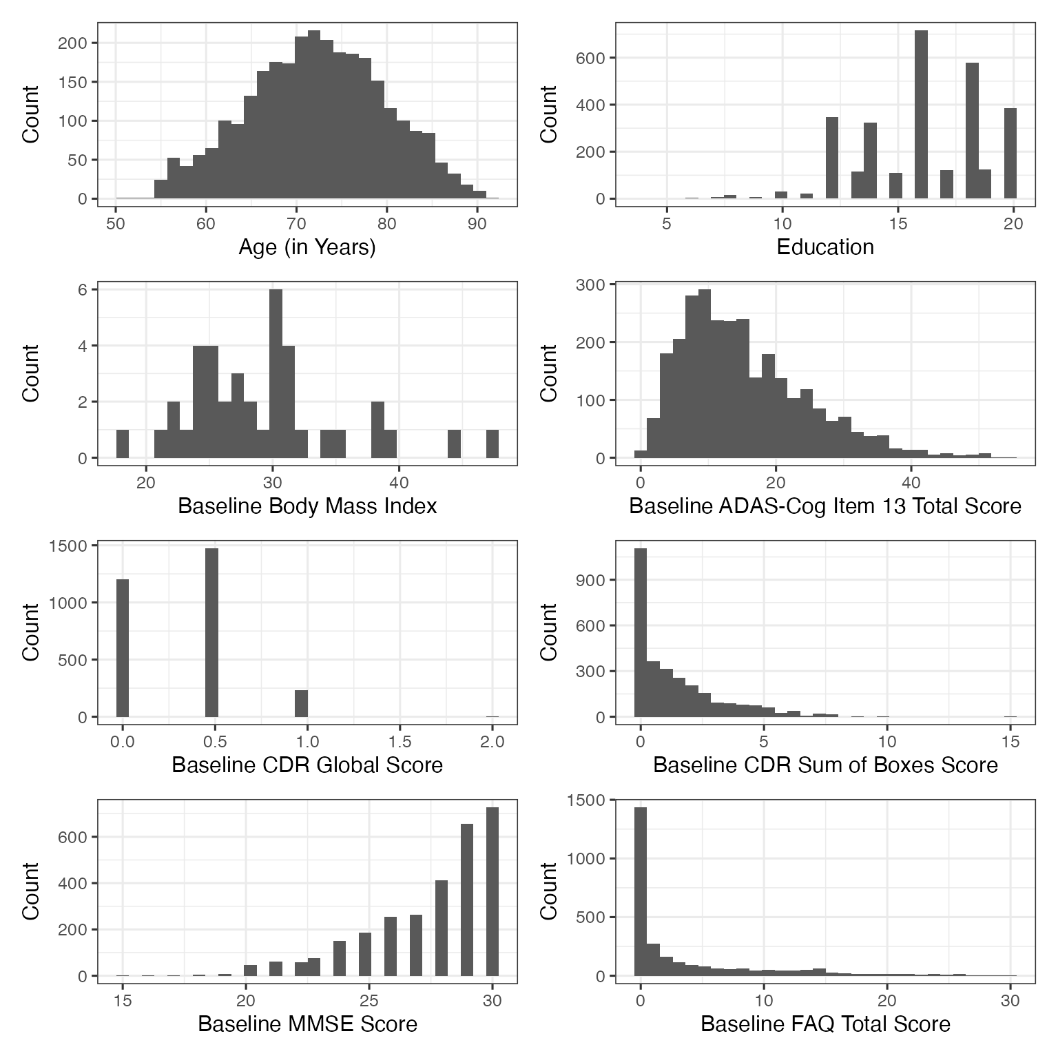
var_label_list <- get_variable_labels(ADSL)
cont_var_list <- c(
  "AGE", "EDUC", "ADASTT13", "CDGLOBAL",
  "CDRSB", "MMSCORE", "FAQTOTAL", "MPACCTRAILSB", "MPACCDIGIT"
)
cont_bl_violin_plot <- lapply(cont_var_list, function(x) {
  graph_data <- ADSL %>%
    filter(ENRLFL %in% "Y") %>%
    rename_with(~ paste0("yvalue"), all_of(x))

  graph_data %>%
    ggplot(data = ., aes(x = yvalue)) +
    geom_histogram() +
    labs(
      x = var_label_list[[x]],
      y = "Count",
      title = paste0("n = ", sum(!is.na(graph_data$yvalue)))
    ) +
    theme(title = element_text(size = 11))
})

names(cont_bl_violin_plot) <- cont_var_list

plots(
  cont_bl_violin_plot,
  n_columns = 2,
  caption = paste0(
    "Baseline mPACCdigit score was based on subjects that were enrolled only ",
    "in ADNI1 study phase. \n The remaining summary plots were based on ",
    "subjects that enrolled in ADNI study."
  ),
  title = "ADNI - Plots of Numeric Characteristics: By Study Phase"
)
Demographic Summaries: By Baseline Diagnostics Status
tbl_summary(
  data = ADSL %>%
    filter(ENRLFL %in% "Y"),
  by = DX,
  include = include_vars,
  type = all_continuous() ~ "continuous2",
  statistic = list(
    all_continuous() ~ c(
      "{mean} ({sd})",
      "{median} ({p25}, {p75})",
      "{min}, {max}"
    ),
    all_categorical() ~ "{n} ({p}%)"
  ),
  digits = all_continuous() ~ 1,
  percent = "row",
  missing_text = "(Missing)"
) %>%
  add_stat_label(label = all_continuous2() ~ conts_statistic_label) %>%
  modify_caption(caption = paste0(
    "Table 2. ADNI - Subject Characteristics: ",
    "By Baseline Diagnosis Status"
  )) %>%
  modify_footnote_header(
    footnote = "Row-wise percentage; n (%)",
    columns = all_stat_cols(),
    replace = TRUE
  ) %>%
  modify_abbreviation(abbreviation = abbrev_list) %>%
bold_labels()| Characteristic |
CN N = 1,2151 |
MCI N = 1,3381 |
DEM N = 4771 |
|---|---|---|---|
| Age (in Years) | |||
| Mean (SD) | 71.0 (7.1) | 72.4 (7.7) | 74.6 (8.0) |
| Median (Q1, Q3) | 70.9 (66.3, 75.9) | 72.7 (66.9, 77.9) | 75.3 (69.8, 80.3) |
| Range | 50.5, 90.3 | 54.5, 91.4 | 55.1, 90.9 |
| (Missing) | 0 | 1 | 0 |
| Sex, n (%) | |||
| Female | 735 (48%) | 582 (38%) | 212 (14%) |
| Male | 480 (32%) | 756 (50%) | 265 (18%) |
| Education | |||
| Mean (SD) | 16.5 (2.6) | 15.9 (2.8) | 15.2 (2.9) |
| Median (Q1, Q3) | 16.0 (15.0, 18.0) | 16.0 (14.0, 18.0) | 16.0 (13.0, 18.0) |
| Range | 6.0, 20.0 | 4.0, 20.0 | 4.0, 20.0 |
| (Missing) | 1 | 2 | 0 |
| Race, n (%) | |||
| American Indian or Alaskan Native | 5 (56%) | 4 (44%) | 0 (0%) |
| Asian | 61 (57%) | 35 (33%) | 11 (10%) |
| Black or African American | 209 (54%) | 140 (36%) | 40 (10%) |
| Native Hawaiian or Other Pacific Islander | 2 (40%) | 3 (60%) | 0 (0%) |
| Other Pacific Islander | 0 (NA%) | 0 (NA%) | 0 (NA%) |
| White | 899 (37%) | 1,124 (46%) | 417 (17%) |
| More than one race | 30 (53%) | 19 (33%) | 8 (14%) |
| Unknown | 9 (39%) | 13 (57%) | 1 (4.3%) |
| Ethnicity, n (%) | |||
| Hispanic or Latino | 105 (54%) | 68 (35%) | 21 (11%) |
| Not Hispanic or Latino | 1,105 (39%) | 1,264 (45%) | 453 (16%) |
| Unknown | 5 (36%) | 6 (43%) | 3 (21%) |
| Marital Status, n (%) | |||
| Divorced | 174 (52%) | 145 (43%) | 18 (5.3%) |
| Domestic Partnership | 8 (62%) | 4 (31%) | 1 (7.7%) |
| Married | 802 (37%) | 977 (45%) | 395 (18%) |
| Never married | 89 (51%) | 67 (38%) | 19 (11%) |
| Unknown | 3 (33%) | 6 (67%) | 0 (0%) |
| Widowed | 139 (44%) | 135 (42%) | 44 (14%) |
| (Missing) | 0 | 4 | 0 |
| APOE Genotype, n (%) | |||
| ε2/ε2 | 5 (56%) | 3 (33%) | 1 (11%) |
| ε2/ε3 | 117 (59%) | 67 (34%) | 14 (7.1%) |
| ε2/ε4 | 22 (35%) | 29 (47%) | 11 (18%) |
| ε3/ε3 | 577 (46%) | 537 (43%) | 129 (10%) |
| ε3/ε4 | 271 (30%) | 430 (48%) | 195 (22%) |
| ε4/ε4 | 37 (15%) | 124 (50%) | 87 (35%) |
| (Missing) | 186 | 148 | 40 |
| Baseline ADAS-Cog Item 13 Total Score | |||
| Mean (SD) | 8.9 (4.4) | 16.4 (6.7) | 29.8 (8.2) |
| Median (Q1, Q3) | 8.3 (5.3, 11.7) | 16.0 (11.3, 21.0) | 29.3 (24.3, 34.3) |
| Range | 0.0, 26.7 | 0.7, 39.7 | 9.3, 54.7 |
| (Missing) | 11 | 19 | 10 |
| Baseline CDR Global Score, n (%) | |||
| 0 | 1,203 (98%) | 23 (1.9%) | 0 (0%) |
| 0.5 | 11 (0.7%) | 1,307 (84%) | 234 (15%) |
| 1 | 0 (0%) | 7 (2.8%) | 240 (97%) |
| 2 | 0 (0%) | 0 (0%) | 3 (100%) |
| (Missing) | 1 | 1 | 0 |
| Baseline CDR Sum of Boxes Score | |||
| Mean (SD) | 0.0 (0.2) | 1.5 (1.0) | 4.4 (1.7) |
| Median (Q1, Q3) | 0.0 (0.0, 0.0) | 1.5 (1.0, 2.0) | 4.5 (3.0, 5.0) |
| Range | 0.0, 2.0 | 0.0, 15.0 | 1.0, 10.0 |
| (Missing) | 1 | 1 | 0 |
| Baseline MMSE Score | |||
| Mean (SD) | 29.0 (1.2) | 27.5 (1.9) | 23.1 (2.3) |
| Median (Q1, Q3) | 29.0 (29.0, 30.0) | 28.0 (26.0, 29.0) | 23.0 (21.0, 25.0) |
| Range | 23.0, 30.0 | 19.0, 30.0 | 12.0, 30.0 |
| (Missing) | 0 | 4 | 1 |
| Baseline FAQ Total Score | |||
| Mean (SD) | 0.2 (1.0) | 3.2 (4.1) | 13.0 (6.9) |
| Median (Q1, Q3) | 0.0 (0.0, 0.0) | 2.0 (0.0, 5.0) | 13.0 (8.0, 18.0) |
| Range | 0.0, 15.0 | 0.0, 24.0 | 0.0, 30.0 |
| (Missing) | 19 | 25 | 4 |
| Baseline mPACCtrialsB | |||
| Mean (SD) | 0.0 (2.6) | -5.3 (3.7) | -13.5 (3.4) |
| Median (Q1, Q3) | 0.3 (-1.7, 1.9) | -5.2 (-8.0, -2.4) | -13.6 (-15.9, -11.2) |
| Range | -12.2, 7.7 | -18.8, 5.1 | -25.3, 0.9 |
| Baseline mPACCdigit | |||
| Mean (SD) | 0.1 (2.4) | -6.9 (3.1) | -13.0 (2.9) |
| Median (Q1, Q3) | 0.2 (-1.2, 1.7) | -7.0 (-9.2, -4.5) | -12.9 (-15.1, -10.8) |
| Range | -5.9, 6.3 | -14.8, 1.6 | -19.5, -5.3 |
| (Missing) | 986 | 941 | 284 |
| Abbreviation: CN: Cognitive Normal; MCI: Mild Cognitive Impairment; DEM: Dementia; SD: Standard Deviation; Q1: the 25th percentile; Q3: the 75th percentile; Baseline mPACCdigit score was based on subjects that were enrolled only in ADNI1 study phase. | |||
| 1 Row-wise percentage; n (%) | |||
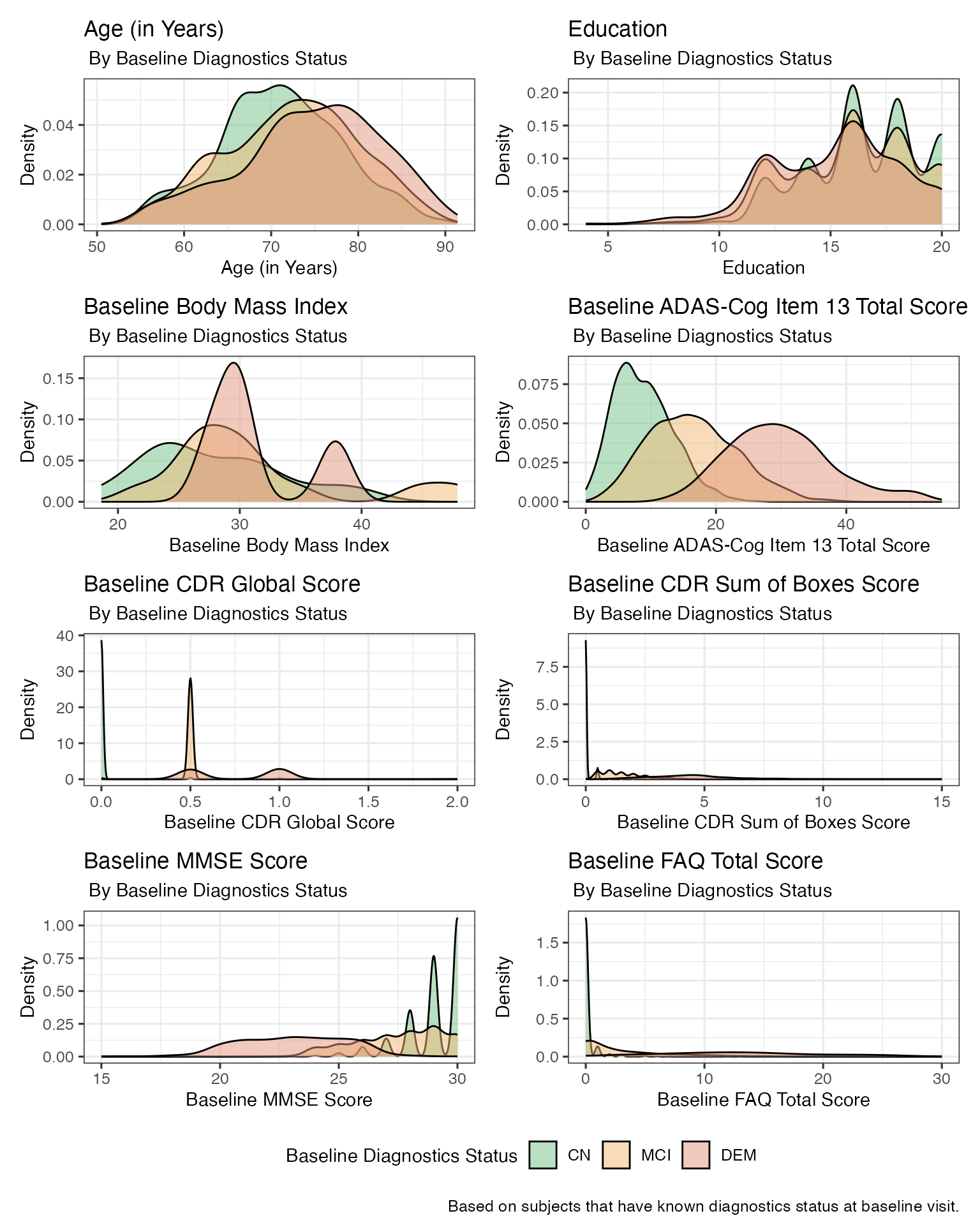
dx_color_pal <- c("#73C186", "#F2B974", "#DF957C", "#999999")

# Create density plot
cont_violin_plot_bl_dx <- lapply(cont_var_list, function(x) {
  graph_data <- ADSL %>%
    filter(ENRLFL %in% "Y") %>%
    filter(!is.na(DX)) %>%
    rename_with(~ paste0("yvalue"), all_of(x))

  n_obs <- graph_data %>%
    select(yvalue, DX) %>%
    na.omit() %>%
    nrow()

  graph_data %>%
    ggplot(data = ., aes(x = yvalue, fill = DX)) +
    geom_density(alpha = 0.5) +
    labs(
      x = paste0(var_label_list[[x]]),
      y = "Density",
      color = get_variable_labels(ADSL$DX),
      title = var_label_list[[x]],
      subtitle = paste0(" By ", get_variable_labels(ADSL$DX), ", n = ", n_obs),
      fill = get_variable_labels(ADSL$DX)
    ) +
    scale_fill_manual(values = dx_color_pal) +
    theme(
      legend.position = "bottom",
      title = element_text(size = 10.5)
    )
})

names(cont_violin_plot_bl_dx) <- cont_var_list

plots(
  cont_violin_plot_bl_dx,
  n_columns = 2,
  guides = "collect",
  caption = paste0(
    "Based on subjects that had known diagnostics status at baseline visit. \n",
    "Baseline mPACCdigit score was based on subjects that were enrolled only ",
    "in ADNI1 study phase. \n The remaining summary plots were based on ",
    "subjects that enrolled in ADNI study."
  ),
  title = paste0(
    "ADNI - Plots of Numeric Characteristics: ",
    "By Baseline Diagnostics Status"
  )
) & theme(legend.position = "bottom")